WO2012151006A1 - Gnss signal processing with delta phase - Google Patents
Gnss signal processing with delta phase Download PDFInfo
- Publication number
- WO2012151006A1 WO2012151006A1 PCT/US2012/029694 US2012029694W WO2012151006A1 WO 2012151006 A1 WO2012151006 A1 WO 2012151006A1 US 2012029694 W US2012029694 W US 2012029694W WO 2012151006 A1 WO2012151006 A1 WO 2012151006A1
- Authority
- WO
- WIPO (PCT)
- Prior art keywords
- rover
- satellite
- anchor
- data
- epoch
- Prior art date
Links
Classifications
-
- G—PHYSICS
- G01—MEASURING; TESTING
- G01S—RADIO DIRECTION-FINDING; RADIO NAVIGATION; DETERMINING DISTANCE OR VELOCITY BY USE OF RADIO WAVES; LOCATING OR PRESENCE-DETECTING BY USE OF THE REFLECTION OR RERADIATION OF RADIO WAVES; ANALOGOUS ARRANGEMENTS USING OTHER WAVES
- G01S19/00—Satellite radio beacon positioning systems; Determining position, velocity or attitude using signals transmitted by such systems
- G01S19/38—Determining a navigation solution using signals transmitted by a satellite radio beacon positioning system
- G01S19/39—Determining a navigation solution using signals transmitted by a satellite radio beacon positioning system the satellite radio beacon positioning system transmitting time-stamped messages, e.g. GPS [Global Positioning System], GLONASS [Global Orbiting Navigation Satellite System] or GALILEO
- G01S19/40—Correcting position, velocity or attitude
- G01S19/41—Differential correction, e.g. DGPS [differential GPS]
-
- G—PHYSICS
- G01—MEASURING; TESTING
- G01S—RADIO DIRECTION-FINDING; RADIO NAVIGATION; DETERMINING DISTANCE OR VELOCITY BY USE OF RADIO WAVES; LOCATING OR PRESENCE-DETECTING BY USE OF THE REFLECTION OR RERADIATION OF RADIO WAVES; ANALOGOUS ARRANGEMENTS USING OTHER WAVES
- G01S19/00—Satellite radio beacon positioning systems; Determining position, velocity or attitude using signals transmitted by such systems
- G01S19/01—Satellite radio beacon positioning systems transmitting time-stamped messages, e.g. GPS [Global Positioning System], GLONASS [Global Orbiting Navigation Satellite System] or GALILEO
- G01S19/03—Cooperating elements; Interaction or communication between different cooperating elements or between cooperating elements and receivers
- G01S19/07—Cooperating elements; Interaction or communication between different cooperating elements or between cooperating elements and receivers providing data for correcting measured positioning data, e.g. DGPS [differential GPS] or ionosphere corrections
-
- G—PHYSICS
- G01—MEASURING; TESTING
- G01S—RADIO DIRECTION-FINDING; RADIO NAVIGATION; DETERMINING DISTANCE OR VELOCITY BY USE OF RADIO WAVES; LOCATING OR PRESENCE-DETECTING BY USE OF THE REFLECTION OR RERADIATION OF RADIO WAVES; ANALOGOUS ARRANGEMENTS USING OTHER WAVES
- G01S19/00—Satellite radio beacon positioning systems; Determining position, velocity or attitude using signals transmitted by such systems
- G01S19/38—Determining a navigation solution using signals transmitted by a satellite radio beacon positioning system
- G01S19/39—Determining a navigation solution using signals transmitted by a satellite radio beacon positioning system the satellite radio beacon positioning system transmitting time-stamped messages, e.g. GPS [Global Positioning System], GLONASS [Global Orbiting Navigation Satellite System] or GALILEO
- G01S19/42—Determining position
-
- G—PHYSICS
- G01—MEASURING; TESTING
- G01S—RADIO DIRECTION-FINDING; RADIO NAVIGATION; DETERMINING DISTANCE OR VELOCITY BY USE OF RADIO WAVES; LOCATING OR PRESENCE-DETECTING BY USE OF THE REFLECTION OR RERADIATION OF RADIO WAVES; ANALOGOUS ARRANGEMENTS USING OTHER WAVES
- G01S19/00—Satellite radio beacon positioning systems; Determining position, velocity or attitude using signals transmitted by such systems
- G01S19/01—Satellite radio beacon positioning systems transmitting time-stamped messages, e.g. GPS [Global Positioning System], GLONASS [Global Orbiting Navigation Satellite System] or GALILEO
- G01S19/03—Cooperating elements; Interaction or communication between different cooperating elements or between cooperating elements and receivers
- G01S19/07—Cooperating elements; Interaction or communication between different cooperating elements or between cooperating elements and receivers providing data for correcting measured positioning data, e.g. DGPS [differential GPS] or ionosphere corrections
- G01S19/072—Ionosphere corrections
-
- G—PHYSICS
- G01—MEASURING; TESTING
- G01S—RADIO DIRECTION-FINDING; RADIO NAVIGATION; DETERMINING DISTANCE OR VELOCITY BY USE OF RADIO WAVES; LOCATING OR PRESENCE-DETECTING BY USE OF THE REFLECTION OR RERADIATION OF RADIO WAVES; ANALOGOUS ARRANGEMENTS USING OTHER WAVES
- G01S19/00—Satellite radio beacon positioning systems; Determining position, velocity or attitude using signals transmitted by such systems
- G01S19/01—Satellite radio beacon positioning systems transmitting time-stamped messages, e.g. GPS [Global Positioning System], GLONASS [Global Orbiting Navigation Satellite System] or GALILEO
- G01S19/13—Receivers
- G01S19/24—Acquisition or tracking or demodulation of signals transmitted by the system
- G01S19/25—Acquisition or tracking or demodulation of signals transmitted by the system involving aiding data received from a cooperating element, e.g. assisted GPS
-
- G—PHYSICS
- G01—MEASURING; TESTING
- G01S—RADIO DIRECTION-FINDING; RADIO NAVIGATION; DETERMINING DISTANCE OR VELOCITY BY USE OF RADIO WAVES; LOCATING OR PRESENCE-DETECTING BY USE OF THE REFLECTION OR RERADIATION OF RADIO WAVES; ANALOGOUS ARRANGEMENTS USING OTHER WAVES
- G01S19/00—Satellite radio beacon positioning systems; Determining position, velocity or attitude using signals transmitted by such systems
- G01S19/38—Determining a navigation solution using signals transmitted by a satellite radio beacon positioning system
- G01S19/39—Determining a navigation solution using signals transmitted by a satellite radio beacon positioning system the satellite radio beacon positioning system transmitting time-stamped messages, e.g. GPS [Global Positioning System], GLONASS [Global Orbiting Navigation Satellite System] or GALILEO
- G01S19/42—Determining position
- G01S19/43—Determining position using carrier phase measurements, e.g. kinematic positioning; using long or short baseline interferometry
Definitions
- PCT/US2010/02563 filed 19 September 2010 (TNL A-2599PCT); International Patent Application PCT/US2010/02562 filed 19 September 2010 (TNL A-2617PCT); International Patent Application PCT/US2010/02581 filed 19 September 2010 (TNL A-2647PCT); United States Provisional
- the present invention relates to the field of Global Navigation Satellite Systems (GNSS). More particularly, the present invention relates to methods and apparatus for processing GNSS data for enhanced Real-Time Kinematic (RTK) positioning.
- GNSS Global Navigation Satellite Systems
- RTK Real-Time Kinematic
- GNSS Global Navigation Satellite Systems
- GLONASS Global Positioning System
- Galileo Galileo
- Compass system the proposed Compass system.
- the rover receiver collects real-time GNSS signal data and receives correction data from a base station, or a network of reference stations. The base station and reference stations receive GNSS signals at the same instant as the rover. Because the correction data arrives at the rover with a finite delay (latency) due to processing and communication, the rover needs to store (buffer) its locally-collected data and time- matches it with the received correction data to form single-difference observations using common satellites.
- the rover uses the single-difference GNSS observations to compute a synchronous position for each epoch using the time -matched data.
- the single-difference process greatly reduces the impact of satellite clock errors.
- satellite orbit errors and atmospheric errors are also reduced by the single-differencing process.
- the need to wait for the correction data means that the synchronous position solution is latent.
- the solution latency includes:
- a prior-art delta phase method used in kinematic survey is aimed at producing low-latency estimates of the rover position without waiting for the matching (synchronous) correction data to be received (see Talbot et. al., Centimeter Accurate Global Positioning System Receiver for On-The-Fly Real-Time Kinematic Measurement and Control, US Patent: 5,602,741, 1 1 February 1997).
- the rover uses them to compute a synchronous position for that epoch.
- the rover estimates its delta position (the rover position difference) from the last synchronous epoch until the current epoch and adds this delta position to the last synchronous position to obtain a current low-latency position estimate while awaiting correction data for a further synchronous epoch.
- the cost of this low-latency scheme is an additional error of about 2-4mm per second of time difference between rover and correction data. The additional error is due mainly to instability of the GNSS satellite clocks.
- FIG. 1 schematically illustrates a scenario using a GNSS rover with correction data for point surveying.
- a user 100 has a rover receiver (rover) 105 which is mounted on a range pole 1 10 or in some cases is a hand- held, or machine-mounted unit without a range pole.
- Rover 105 includes a GNSS antenna 1 15 and a communications antenna 120.
- Rover 105 receives at its GNSS antenna 1 15 the signals from GNSS satellites 125, 130, 135, 140, 145, etc.
- Rover 105 also receives at its communications antenna 120 correction data from a corrections source 150 via a communications link 155.
- the communications link is, for example, a radio link or mobile telephone link, or any other suitable means of conveying the correction data to the rover 105.
- the correction data can be of any suitable type for improving the positioning accuracy of rover 105, such as: differential base station data from a base station serving as corrections source 150, or virtual reference station data from a network of reference stations serving as corrections source 150 (WAAS is one example), or precise orbits and clocks data from a Precise Point Positioning (PPP) service such as that described in United States Provisional Application for Patent No. 61/277, 184 filed 19 September 2009 (TNL A- 2585P) and in International Publication Number WO 201 1/034616 A2 dated 24 March 201 1 (TNL A- 2585PCT).
- PPP Precise Point Positioning
- FIG. 2 is a block diagram of a typical integrated receiver system 200 with GNSS antenna 1 15 and communications antenna 120.
- Receiver system 200 can serve as rover 105 or as a base station or reference station.
- Receiver system 200 includes a GNSS receiver 205, a computer system 210 and one or more communications links 215.
- Computer system 210 includes one or more processors 220, one or more data storage elements 225, program code 230 for controlling the processor(s) 220, and user input/output devices 235 which may include one or more output devices 240 such as a display or speaker or printer and one or more devices 245 for receiving user input such as a keyboard or touch pad or mouse or microphone.
- the program code 230 is adapted to perform novel functions in accordance with embodiments of the invention as described below.
- the integrated receiver system 200 can otherwise be of a conventional type suited for mounting on a range pole or for hand-held operation; some examples include the Trimble R8 GNSS, Trimble R7 GNSS, Trimble R6 GPS and Trimble 5700 surveying systems and the Trimble GPS Pathfinder Pro XRS system.
- FIG. 3 illustrates the error in the height component of synchronous RTK position estimates: 300, 301, 302, 303, ... 308, for epoch times 0.0, 1.0, 2.0, 3.0, ... 8.0 seconds respectively.
- the RTK position fixes: 300, 301, 305, & 306 are considered fixed i.e. have carrier phase ambiguities that are essentially resolved to integer values.
- the RTK position fixes at: 302, 303, 304, and 308, are considered float solutions, i.e., the carrier phase ambiguities cannot be resolved to integer values. Note that at time 7.0s, there is no RTK position solution.
- the precision (uncertainty) of each RTK position fix is represented by a vertical error bar.
- Autonomous (point position) solutions are produced by the rover GNSS receiver at say a 10Hz rate. For clarity, just the 1 Hz autonomous height estimates are shown in Error! Reference source not found., while the intervening autonomous heights are illustrated with a dashed line.
- the autonomous lHz height estimates are: 310, 31 1, 312, 313, ... 318, corresponding to epoch times: 0.0, 1.0, 2.0, 3.0, ... 8.0s respectively.
- Autonomous position estimates generally have a precision of several decimeters up to several meters.
- FIG. 4 illustrates the timing of various events relevant to delta phase processing.
- Time axis 350 represents actual time, with values shown from 1.0s through to 3.0s.
- the rover GNSS receiver measurements are sampled and made available for processing a short time after the actual time.
- the rover measurements for epoch 1.0s are available at event 361.0; the rover measurements for epoch 1.2s are available at event 361.2; and so on, as shown on axis 360.
- Axis 370 corresponds to the time that correction data is received at the rover.
- the correction data must first be sampled by a real reference station, or a network of reference stations, before being sent and received by the rover, therefore there is an inherent latency in the received correction data.
- Event 371 corresponds to the receipt of correction data for epoch Is; event 372 corresponds to the receipt of correction data for epoch 2s.
- the rigorous satellite orbit and clock data is normally derived from a network of spatially distributed reference stations (e.g. a regional, or global network).
- the network GNSS observations must first be concentrated at a central facility, then processed and finally formatted and distributed to one or more rovers.
- the rigorous satellite orbit and clock data is often old by the time it reaches the rover(s).
- GNSS Processing with Predicted Precise Clocks [TNL A-2796] [0017] Positioning methods and apparatus are presented which use predicted precise GNSS satellite clock error models.
- GNSS data are derived from signals received at a rover antenna. At least one of correction data and rigorous satellite data are obtained. A time sequence is maintained of at least one rover position and at least one rover position difference with associated time tags. The time sequence is used to determine at least one derived rover position. The derived rover position is reported.
- a set of GNSS satellite clock error models is maintained. The time sequence is extended upon arrival of rover data associated with a new time tag. At least one clock error model is updated upon arrival of rigorous satellite data.
- Positioning methods and apparatus which use mixed-quality data.
- GNSS data derived from signals received at a rover antenna are obtained.
- At least one of correction data and rigorous satellite data is obtained.
- a time sequence is maintained, of at least one rover position and at least one rover position difference with associated time tags.
- the time sequence is obtained by estimating at least one position difference using rigorous satellite data from multiple satellites using at least two combinations of data selected from: for at least one satellite, no correction data and broadcast satellite data; for at least one satellite, no correction data and rigorous predicted satellite data, for at least one satellite, no correction data rigorous satellite data for said at least one satellite; for at least one satellite, correction data and broadcast satellite data; for at least one satellite, rigorous predicted satellite data and correction data; and for at least one satellite, rigorous satellite data and correction data.
- the time sequence is used to determine at least one derived rover position. The derived rover position is reported.
- Positioning methods and apparatus are presented which maintain a time sequence.
- GNSS data derived from signals received at a rover antenna are obtained.
- At least one of correction data and rigorous satellite data are obtained.
- a time sequence of at least one rover position and at least one rover position difference with associated time tags is maintained.
- the the time sequence is extended with a computed synchronized position upon arrival of correction data
- At least a portion of the time sequence is modified upon arrival of one of correction data and rigorous satellite data.
- the time sequence to determine at least one derived rover position.
- the derived rover position is reported.
- the low-latency position estimates are based on an accumulation of delta positions and the last available synchronous position fix. Each time a new synchronous position fix is available, there is generally a jump in the reported low-latency position fixes.
- the magnitude of the low-latency position fix jumps is mostly due to the precision of the underlying synchronous position solutions. It is desirable in many applications to produce high update (> lHz) position fixes that are not affected by discontinuities caused by jumps in the synchronous position fixes. In particular machine guidance applications benefit from smooth and continuous position input to the control system(s).
- a respective synchronous position to be propagated to an anchor epoch is obtained for each epoch of a set of at least one epoch.
- the respective synchronous position is combined with at least one rover position difference defining a change of rover position from the epoch of the respective synchronous position to the anchor epoch, to obtain a respective propagated position for the anchor epoch.
- at least one propagated position for the anchor epoch is blended with the synchronous position for the anchor epoch to obtain a blended anchor position for the anchor epoch.
- a propagated rover position is determined for a current epoch by combining the blended anchor position with at least one rover position difference defining a change of rover position from the anchor epoch to the current epoch.
- the switch in physical reference station therefore typically leads to a switch from fixed, high quality position solution, to a period of float, low quality position solution, immediately following the physical reference station change.
- Many high-precision GNSS applications require utmost (cm-level) accuracy and therefore need to wait until the fixed solution quality returns following the physical reference station change. It is advantageous to be able to bridge reference station changes with delta phase processing.
- GNSS data derived from signals received at a rover antenna are obtained.
- Correction data are obtained.
- a time sequence of at least one rover position and at least one rover position difference with associated time tags is maintained. The time sequence is used to determine at least one derived rover position by, starting from a position determined using corrections synchronous with rover data as an anchor position at a time tag, deriving a new anchor position for the time tag of the anchor position and at least one other estimated rover position at the time tag of the anchor position.
- the new anchor position at the time tag is reported as the rover position at a time associated with the time tag of the anchor position, or the new anchor position at the time tag of the anchor position is combined with at least one rover position difference to determine a new derived rover position for a subsequent time tag, and the new derived rover position is reported as the rover position at a time associated with the subsequent time tag.
- the autonomous position of the rover is used as the linearization point for the delta position computations.
- the autonomous position of the rover is in error by several decimeters, up to several meters. Large errors in the linearization point leads to a proportional error in the output delta position estimates. The linearization errors accumulate with propagation time, therefore large correction data latency causes increased error growth in the delta position estimates.
- Methods and apparatus for processing of GNSS signal data are presented. An approximate rover anchor position for a first epoch is obtained. The approximate rover anchor position is used to determine a rover position difference for at least one succeeding epoch. An improved rover anchor position is obtained for the first epoch.
- An adjusted rover position difference is derived for each of these succeeding epochs.
- a rover position for a current epoch is derived from the improved rover anchor position for the first epoch and at least one adjusted rover position difference.
- FIG. 1 schematically illustrates a scenario using a GNSS rover with correction data for point surveying
- FIG. 2 is a block diagram of an integrated GNSS receiver system
- FIG. 3 illustrates the error in the height component of synchronous RTK position estimates
- FIG. 4 illustrates the timing of various events relevant to delta phase processing
- FIG. 5 illustrates an orbiting GNSS satellite
- FIG. 6 describes the processing steps required to form a rover position difference between two epochs
- FIG. 7 illustrates a rover receiver at two consecutive epochs
- FIG. 8 is a block diagram illustrating components of a GNSS data processing scheme
- FIG. 9 shows true rover positions at a first and a second epoch
- FIG. 10 is a flowchart of a procedure for adjusting delta position estimates for errors in initial coordinates
- FIG. 1 1 depicts adjustment for initial position errors
- FIG. 12 illustrates a 10Hz rover position difference trajectory
- FIG. 13 illustrates a 4s rover position difference trajectory
- FIG. 14 illustrates relative uncertainties of various solutions types over time
- FIG. 15 presents timeline views of positions (height component only) derived from various techniques
- FIG. 16 presents a flowchart that explains the handling of data at a rover.
- FIG. 17 shows an expanded view of the flowchart of FIG. 16.
- Delta phase is defined here as being the difference in carrier phase observed to a GNSS satellite over a specific time interval.
- GNSS carrier phase measurements observed by a receiver to a GNSS satellite have millimeter precision, however the measurements are affected by a number of biases. If carrier phase tracking is maintained, the delta phase measurements give a precise measure of the change in range (distance) between user and satellite over time.
- the user is located at positions U(l) and U(2), denoted 415 and 420, at times t(l) and t(2) respectively.
- the ranges from user to satellite at the two epochs are R(l) and R(2) respectively.
- the observed phase measurements ⁇ (1) and ⁇ (2) are free from errors and therefore are equal to the true ranges R(l) and R(2) respectively.
- the delta phase measurement (in units of meters), for epoch 1.0s to 2.0s, is defined as:
- ran e at epoch k
- the ran e is related to the user and satellite coordinates via the following:
- the satellite coordinates S(k) [ X(k), Y(k), Z(k) ] are known from a broadcast or rigorous satellite ephemeris.
- the user coordinates U(k) [ x(k), y(k), z(k) ] are the only unknown quantities in (3). If delta phase is observed to at least 3 satellites, the corresponding change in user location can be derived for the same time interval. In practice, a forth satellite must be observed in order to estimate the change in receiver clock over the delta phase time interval. [0041 ] Delta phase observation equation
- the single receiver phase observation equation forms the basis of the delta phase observation equation and therefore is presented first.
- the following single receiver phase observation equation applies to a single receiver observation to a single satellite:
- ⁇ ( ⁇ ) R(k) + T(k) + P(k) - T(k) + ⁇ k) + + atk) + N (4)
- N integer carrier phase ambiguity term
- Equation (4) the satellite index is omitted in Equation (4).
- the delta phase observation equation is formed by differencing (4) with respect to time:
- S0(k,l) S0(l) - S0(k) ⁇ SR(k, /) + ST(k, /) + SP(k, /) + Sr(k, /) + Sfiik, /) + + Sco(k, /)
- a Taylors series expansion can be used to linearly relate the unknowns to the observations:
- ⁇ , /) / ⁇ 5c (/), y(l), z (/), Sr(k, /) ⁇
- G(k, /) (4xs) gain matrix which relates a change in a measurement to a change in the estimated parameters.
- Rover position differences only provide an estimate of the relative trajectory of the rover over time.
- An anchor position absolute position
- the anchor position normally takes the form of a synchronous position, derived from processing single- difference rover and correction data in a filtering scheme that estimates rover position, phase ambiguities and other nuisance parameters.
- DGPS synchronous position
- inertial navigation systems etc.
- FIG. 6 describes the processing steps required to form a rover position difference between two epochs.
- Table 1 illustrates a time sequence of rover position differences buffered for high rate (say 5Hz) delta phase processing.
- Table 2 illustrates a time sequence of rover position differences buffered for low rate (IHz) delta phase processing. Note that the time sequences are normally implemented as circular buffers, indexed with time.
- carrier phase observations generated at the rover are time-differenced w.r.t. to the last data epoch t(k). Note that only those satellites that were continuously tracked are used in the formation of delta phase observations;
- the approximate rover position at the current epoch U'(l) [x(l), y(l), z(l)] is taken from the rover receiver autonomous position solution, or differential position solution.
- the approximate current position U'(l) [x(l), y(l), z(l)] is used to generate coordinate partials [see (6)-(10)] for each measurement. While the approximate current and first epoch positions are used in the formation of the computed (theoretical) delta phase measurement for each satellite. The precision of the approximate rover coordinates is dependent on the source. For example autonomous position estimates are generally good to meter-level, although in poor tracking environments tens of meters of error may result. Inaccuracies in the approximate positions lead to errors in the computed delta position, which is explained in detail later.
- the most-probable rover position difference and receiver clock drift are computed using least squares (12) or comparable estimation methods.
- the time sequence buffers may include:
- FIG. 7 Error! Reference source not found.illustrates a rover receiver at two consecutive epochs 615 and 620 respectively, tracking a single satellite.
- the satellite moves along orbit 630 and is located at 605, denoted S(l), at epoch 1, and 610, denoted S(2), at epoch 2.
- a stationary reference receiver 600 denoted B, tracks the same satellite as the rover.
- the location of the reference receiver is given in Cartesian coordinates as ( ⁇ ⁇ , ⁇ ⁇ , ⁇ ⁇ ).
- Carrier phase measurements observed at the rover are given by ⁇ (1) and ⁇ (2), for epochs 1 and 2 respectively.
- the corresponding user-satellite ranges are given by Ru(l) and Ru(2) respectively.
- Carrier phase measurements observed at the reference are given by ⁇ ⁇ (1) and ⁇ ⁇ (2) for epochs 1 and 2 respectively; with corresponding user-satellite ranges: R B (1) and R B (2) respectively.
- ⁇ indicates a difference operation between reference (B) and rover (U) quantities.
- the receiver clock drift parameter estimated is in fact the drift of the difference between rover and reference/correction clocks. In principle this does not imply any changes in the set-up of the computation of the position differences.
- the weight matrix modified from (1 1) is thus:
- the latest GPS satellites broadcast coherent carriers on LI, L2 and L5 frequency bands.
- GLONASS satellites broadcast on two bands near GPS LI and L2. All planned GNSS signal structures include at least two bands per satellite.
- Multi-frequency carrier phase measurements are often combined into various linear combinations with particular properties.
- the wide-lane GPS L1/L2 phase combination has an effective wavelength of 86cm making it useful for ambiguity resolution purposes.
- the iono-free phase combination is particularly useful for (essentially) removing the effect of ionospheric bias.
- the ionosphere presents a significant source of error in delta phase processing therefore the iono-free phase combination is particularly useful for delta phase positioning.
- the position calculations are normally performed at the rover receiver.
- the rover data is available within a fraction of a second after being sampled by the receiver.
- the correction data must be sampled, formatted, transmitted, received and decoded before it can be used for processing at the rover.
- the latency of the correction data is typically 1 -60s, depending on the type of data link used.
- There are many high-precision applications where the location of the rover is required with very small latency. For example machine control where a cutting implement is driven to a design surface in real-time.
- Low latency RTK positioning can be achieved by combining single-receiver (rover) delta phase measurement processing with latent synchronous (base-rover) position solutions.
- FIG. 8 presents a block diagram illustrating the various components of a GNSS data processing scheme.
- the rover GNSS data, 650 is prepared at 654.
- the GNSS correction data 652 is prepared at step 656.
- the prepared rover and correction data are time matched and used to form single- difference GNSS observations 664, using the Single Difference Builder 658.
- the prepared rover data (654) is applied to the single-receiver delta phase processor 660, to produce a time sequence of rover position differences 662.
- the single-difference GNSS data 664 is used by the synchronous processor 666 in an estimation scheme (e.g., least squares estimator or Kalman filter) to estimate the rover position as well as carrier phase ambiguity and other nuisance parameters.
- the output of the synchronous processor 666 is synchronous positions 668.
- the single-difference GNSS data 664 is also used in the single-difference delta phase processor 670, to produce a time sequence of rover receiver (single-difference) position differences (672).
- the rover position difference time sequence (662), synchronous positions (668) and single-difference rover position difference time sequence 672 are optionally combined in Blender 674 to produce the reported position 676.
- Table 3 provides an illustration of the process used to construct reported position based on synchronous position and rover position difference estimates.
- the correction data latency is 1 s and the data update rate is 5Hz.
- the first delta phase epoch occurs at 1.2s, when the two consecutive data epochs are available. Only rover position differences are available up until the first synchronized position fix is produced at epoch 2.0. Once synchronized position fixes are available, the reported position is constructed from the accumulation of rover position differences and the last synchronous fix. One Hz delta positions are used to propagate the synchronous positions across multiple seconds.
- each delta phase measurement will be different for each satellite tracked at the same epoch. Also the delta phase measurement variances will vary for each satellite over time. Satellites that are low on the local horizon tend to be more affected by atmospheric errors and multipath, therefore satellites low on the horizon are assigned larger tropospheric, ionospheric and multipath variances. Furthermore, the signal strength is worse near the horizon and therefore the uncorrected measurement noise is worse.
- Satellites with rigorous orbit and clock information can be processed with those satellites tracked at the same epoch that only have broadcast information. It is important to supply the appropriate a-priori measurement variances when mixing satellite observations derived from rigorous and broadcast sources.
- the low-latency reported position is given as the sum of a number of delta position epochs, combined with the last synchronous position (see the example in Table 4, extracted from Table 3).
- ⁇ d ⁇ (k,l) ( ⁇ ST(k ) + &dP(k,l) + ⁇ , ⁇ ) + &Sp(k,l) + &&(k,l) + ⁇ ⁇ 5 (k,l) (23) [0107] At each delta phase measurement epoch, the following two position uncertainties are computed:
- Equation (18) is the standard formula for computing the delta phase position uncertainty. Whereas, just the time -wise errors are considered in the delta position uncertainty calculation in (24).
- the International GNSS Service generates rigorous network predicted orbits based on GNSS data from globally distributed tracking stations.
- the IGS refers to their rigorous-network predicted orbits as Predicted Precise Orbits. Their Predicted Precise Orbit?, are made available for download via the Internet (see Kouba, A Guide to Using International GPS Service (IGS) Products. Geodetic Survey Division, Natural Resources Canada, February 2003,
- 2585PCT include a detailed explanation of an apparatus/method for estimating rigorous orbits and clocks based on a Global satellite tracking network. Parts 8 and 9 thereof document the estimation of rigorous orbits and clocks respectively.
- 201 1/126605 A2 dated 13 October 201 1 (TNL A-2633PCT) describes how global and regional GNSS tracking stations are used together with network processing software for estimating rigorous orbit and clock corrections.
- the system delivers GNSS satellite orbits with a precision of around 5cm, and an update rate of 10s.
- Rigorous clock information is generated and is provided to rover receivers at a rate of 2s.
- the combination of rigorous orbit and clock information means that the error growth for single- receiver delta phase positioning is bounded.
- T k satellite clock error at epoch k for satellite s
- f k satellite clock drift at epoch k for satellite s
- a Kalman filtering scheme can be applied to the models defined by Equations (26), (27) and (28), with one filter per satellite.
- a prediction of the satellite clock error is made based on the filtered satellite clock error and satellite clock drift according to: where the accent ⁇ indicates a predicted quantity, and accent ⁇ represents a filtered quantity.
- the predicted clock error T s (k) for each satellite is used in the right-hand side (RHS) of (4) to correct the delta phase measurements.
- a clock predictability number can be generated for each satellite by studying the magnitude of prediction errors due to various prediction lengths up to a predefined interval of say two minutes. The largest difference between the predicted clock correction and estimated one provides the predictability number:
- the predictability numbers p l s 2 o(k) for good satellites are typically below 0.25m, for a regular satellite it is between 0.25m and 0.5m, for a bad satellite it's between 0.5m and 0.75m. If the number is above 0.75m the satellite should not be used for predictions. Most of the GPS and nearly all GLONASS satellites have numbers below 0.25m.
- Satellite clock quality indicators can be produced either by the network software or by the rover(s).
- the clock quality indicators are used in the apriori noise model of the rover receiver delta phase processor. Satellites with highly predictable clocks are therefore given more weight (smaller
- Satellite clock drift Dependent on the stability of the satellite clock. Satellite atomic frequency standards have long term stabilities of ⁇ lO 2 . The satellite clock drift rate must be scaled by the speed of light to determine the impact on the delta phase measurements. The unmodelled satellite clock drift rate causes several millimeters / second error in delta phase positioning.
- Satellite orbit error Broadcast GPS orbits have a precision of l-5m; while
- GLONASS satellites are slightly worse. Rigorous orbits are good to around 2-5cm. Satellite orbit errors cause a drift in the delta phase position estimates which is dependent on the magnitude of the satellite position error.
- the tropospheric bias term refers to the unmodelled part of the tropospheric error rate. Generally the tropospheric bias changes slowly (over tens of minutes), however passing weather fronts cause a faster rate of change of say 10-50mm / minute.
- Ionospheric bias The rate of change of the unmodelled ionospheric bias is on the f 2 order of say 5-20mm/s for low elevation satellites and less for high-elevation satellites (under stable ionospheric conditions).
- the iono bias is a significant error source for delta phase processing.
- the ionospheric bias can be obviated using iono-free delta phase processing.
- Multipath bias The rate of change of the carrier phase multipath is typically 5- 20mm / minute for low-elevation satellites and much less for high elevation satellites (which are generally less affected by signal reflections). Multipath bias is cyclic in nature and is generally ⁇ 5cm in magnitude.
- Table 6 provides a summary of the magnitude of errors affecting single-receiver and single- difference delta phase observations.
- single-receiver delta phase positioning all satellite and atmospheric errors directly impact on rover position difference estimates.
- single-difference delta phase processing the closer the separation of base and rover the less the impact of orbit and atmospheric errors on the estimated rover position difference.
- Satellite orbit error broadcast orbit broadcast orbit :
- Tropospheric bias 5.0e-6 to 1.0e-3 m/s B*5.0e-6 to B* 1.0e-3 m/s
- Ionospheric bias 1.0e-3 to 0.02 m/s B*0.001 to B*0.02 m/s
- Table 7 summarizes the errors affecting single-receiver delta phase processing based on rigorous orbit / clock correction data. Note that the satellite clock drift and orbit errors only accumulate until the next satellite clock/orbit correction message is received. Also note that the ionospheric bias is normally zero since iono-free delta phase processing is used. The remaining errors are due to unmodelled tropospheric bias and carrier phase multipath, both of which change relatively slowly over time.
- the true rover positions at the first and second epoch are 710 and 715, denoted U(l) and U(2) respectively.
- the corresponding true ranges for the first and second epoch are R(l) and R(2) respectively.
- the true user position is not known, but rather approximate user positions are obtained from, e.g., autonomous or differential GNSS solutions.
- A(/)] reflects the geometry change between both epochs mainly caused by motion of the satellites and has to be computed in parallel to the initial delta-position estimation using the approximate initial position. For each delta-position estimate, the approximate previous epoch position
- FIG. 10 contains a flowchart which summarizes the procedure used to adjust delta position estimates for errors in initial coordinates.
- the following example illustrates the position adjustment process: [0100]
- a synchronous position becomes available for epoch 1.0s (i.e. we have ⁇ (1.0) ).
- the synchronous (anchor) position is known to be accurate to say a few centimeters in a global sense.
- the time sequence (rover delta position difference) buffer is scanned in steps 805 and 810 until a matching interval is found with starting time 1.0s and end time 2.0s.
- the adjusted rover position difference for epoch 2.0 is then computed at 825 and is given by the saved (and slightly biased) rover position difference, plus the correction for initial position error:
- the adjusted position for epoch 2.0 is produced at 830 based on:
- ⁇ (2. ⁇ ) ⁇ ( ⁇ . ⁇ ) + ⁇ ( ⁇ .0,2.0)
- step 835 A test is made at step 835 to see if the adjustment process is complete for all epochs.
- the current time is 3.0s, hence steps 3-6 must be repeated for the time interval 2.0 - 3.0s.
- ⁇ (2.0,3.0) ⁇ (2.0,3.0) + ⁇ (2.0,3.0)
- ⁇ (3.0) ⁇ (2.0) + ⁇ (2.0,3.0)
- FIG. 1 1 Error! Reference source not found.depicts the adjustment for initial position errors.
- just the height component of a stationary rover is considered.
- hollow circles correspond to autonomous height estimates at each measurement epoch (920).
- Grey lines indicate rover position difference height estimates. Note that the further the initial height is away from the correct height, the larger the error in the rover position difference height estimate. Also note that the rover position difference height estimates are affected in this example by both the systematic effect of initial height error, plus the random delta phase measurement errors.
- the trace in sub-graph 905 is obtained by first shifting the rover position difference height estimate for t(l .0, 1.1) to join with the synchronous position height at t(l .0). Next the rover position difference height estimate t(l.1-1.2) is linked to the previous position at t(l . l), and so on until the next synchronous position height is available, in this case at t(2.0).
- the synchronous position height estimates contain small errors and therefore discontinuities exist when linking delta positions with synchronous positions.
- rover position difference estimates are normally generated at say 5, 10 or 20Hz. Typically the rover position difference estimates form a smooth trajectory. Small jumps sometimes occur with changes in satellites geometry, i.e. new satellites entering the solution, or satellites being lost. As implied by the name, rover position difference estimates only provide relative changes in user location over time. The absolute position of the user is required at an epoch to be able to anchor the rover position differences. Synchronous position estimates derived from a position + ambiguity processor are normally used in conjunction with delta phase processing to produce low- latency position estimates.
- Measurement errors lead to variations in the synchronous position estimates, which in turn leads to discontinuities in the reported position trajectory.
- FIG. 12 illustrates a 10Hz rover position difference trajectory 1005, from time 1.0 to 4.0s. Just the height component is shown. Synchronous position solutions are generated at lHz and are illustrated as solid black circles 1010, 1020, 1030 & 1040.
- the rover position difference trajectory 1005 is first adjusted to the synchronous position 1010, at 1.0s. When the next synchronous position is available for 2.0s, 1020, the rover position difference trajectory is shifted by 1045, to 1060. Trajectory 1060 is again shifted based on the synchronous position 1030, at 3.0s, to form 1070. This adjustment process is repeated at 4.0s, and so on.
- a step in the rover position difference trajectory occurs for each synchronous position adjustment. Note that the magnitude of the stepping effect has been exaggerated for the purposes of this example.
- FIG. 13 illustrates a 4s rover position difference trajectory (1 105). Synchronous positions are obtained at times 1,2,3 & 4s, denoted 1 1 10, 1 120, 1 130 & 1 140 respectively. Comparisons can be made between the rover position difference estimates at lHz epochs (1 1 15, 1 125 & 1 135) with the corresponding synchronous position estimates (1 120, 1 130 & 1 140), thus leading to the differences 1 145, 1150 and 1 155, respectively. Rather than introducing abrupt steps in the reported position trajectory, it is possible to blend the rover position difference trajectory with the synchronous positions.
- the blending process involves the following steps:
- a weighting factor is generated for the anchor epoch synchronous position and a weighting factor is generated for the older synchronous position, propagated to the anchor epoch.
- a blended anchor position is generated from the anchor epoch synchronous position and the older synchronous position propagated to the anchor epoch.
- multiple synchronous positions, propagated to the anchor epoch can be used in the blending process.
- the number of synchronous positions considered in the blending process is a design parameter.
- a buffer of the last n synchronous position fixes is maintained, as well as a buffer of the last n corresponding rover position difference estimates.
- Table 8 provides an example of the position buffering and blending process for the example given in FIG. 13Error! Reference source not found..
- the synchronous positions are shown in column 2 as: U(1.0), U(2.0), U(3.0) & U(4.0).
- Delta phase processing yields rover position differences: U(l .0,2.0), U(2.0,3.0), U(3.0,4.0) as shown in column 3.
- (a,b) are used to weight the synchronous solution and propagated synchronous positions at the anchor epoch.
- (a,b) ] determines the characteristics of the blended solution. Normally the most recent synchronous position is given the most weight, while the oldest position the least weight. A linear, exponential or other suitable, weighting scheme can be used.
- the raw precision-based blending factors are given by:
- the physical reference station changes in a network data stream, which normally causes a reset in the synchronous position processor and an interruption to the position report, followed by a period of float-quality positioning.
- FIG. 14 provides an illustration of the relative uncertainties of various solutions types over time assuming all solution types use the same satellite geometry.
- the axis 1205 corresponds to fixed- quality synchronous solutions, with each position 1230, identified with solid black dots.
- the uncertainty of the positions is represented by error bars 1235.
- the float-quality synchronous positions on axis 1210 have larger uncertainty than the fixed- quality synchronous solutions, as evidenced by the longer error bars 1245.
- Each float-quality synchronous position, 1240 shows larger variations about the zero axis, 1210.
- the precise single-receiver rover position difference positions are presented on axis 1220. Each position fix is marked by a black ring (1260). The error growth of the precise rover position difference estimates is shown as the region 1265, assuming that the propagation time starts at first epoch and accumulates thereafter.
- the predicted-precise single-receiver rover position differences are presented on axis 1222. Each position fix is marked by a dark grey circle surrounded by a black ring (1262). The error growth of the predicted-precise rover position difference estimates is shown as the region 1267.
- the single-receiver rover position differences (broadcast orbits and clocks) is shown on axis 1225, with each position fix marked by a grey ring.
- the error growth of the single -receiver rover position differences is defined by the region 1275.
- the time -wise error growth of single-difference rover position difference is lower than that of the precise (single -receiver) rover position difference; which is lower than the predicted-precise rover position difference; which is lower than the single -receiver rover position difference (broadcast orbits and clocks).
- Single-difference processing requires reference and rover receivers to be tracking common satellites.
- FIG. 15 presents timeline views of positions (height component only) derived from prior art and new techniques.
- the upper axis 1305, refers to prior-art positioning methods, while the lower axis, 1310, to new techniques.
- the position trace for axis 1305 is denoted 1315; for axis 1310, the position trace is denoted 1320.
- the prior-art method axis 1305), during times 1-2, the solution has fixed quality.
- this event causes the synchronous processor to reset. This results in a period of float quality synchronous positioning up until epoch 6. During the float period, the accuracy of the reported position is only decimeter-level. At epoch 6, the synchronous fixed quality is reestablished (segment 1350) and retained until reference station corrections are lost just after epoch 7. The float quality solutions are propagated using single-receiver delta positions through segment 1355.
- FIG. 16 presents a flowchart that explains the handling of data at the rover. When new data arrives at 1505, it is tested at 1510 to see if it is rover data. If so, rover data handling occurs at 1525.
- Test 1515 checks for the presence of Precise Orbit and Clock information. When present, the Precise Orbits and Clocks are handled at 1530. The input data is tested at 1520 to see if it is from the reference and can be single- differenced. If so, the single-difference data is handled at 1535.
- FIG. 17 shows an expanded view of flowchart 1500.
- rover data When rover data is received, it is used to form a rover position difference solution between the current and previous epoch (1605).
- the rover position difference estimate is then buffered at step 1610, and optionally used to generate a low- latency position estimate at 1612.
- the rigorous predicted satellite clock/orbit models are updated at 1613.
- the rigorous predicted clock/orbit information is optionally used at 1614 to update the rover position difference for the current data epoch.
- the rigorous predicted orbit information is used to update the time sequence of rover position difference estimates.
- the best rover position difference time sequence is generated at 1616 based on the predicted precise rover position difference time sequence and existing broadcast rover position difference time sequence.
- the best rover position difference from 1616 is used to replace the predicted rover position difference time sequence at 1617.
- the rigorous satellite clock/orbit models are updated at 1620, as soon as rigorous orbit and clock information is received for one or more satellites.
- the rigorous clock models enable the rover position difference time sequence derived from broadcast clocks to be optionally refined (1625) and stored.
- the rigorous orbit and clock information is used to form a precise rover position difference estimate for the current and previous epochs at 1630.
- the best rover position difference time sequence is produced based on the existing precise position sequence.
- the predicted rover position difference time sequence is replaced by the rover position difference time sequence with the smallest error.
- a synchronous position result is produced at 1660, using the latest single-difference GNSS measurements.
- the best (smallest uncertainty) synchronous position solution is derived from the latest synchronous position result, and the single-difference rover position difference time sequence in step 1665. If for example the synchronous position result is float quality, then often the single-difference rover position difference time sequence that was propagated from the last fixed quality solution will be the best (smallest uncertainty).
- all of the single-difference rover position differences up to the reference data time tag are replaced with the new synchronous position solution.
- an optional report of the synchronous position is provided which will be latent with respect to the current time.
- a positioning method comprising:
- maintaining a set of GNSS satellite clock error models further comprises, upon arrival of rigorous satellite orbit and clock data, updating the time sequence.
- the set of satellite clock error models comprises up to one clock error model per satellite.
- the correction data comprises at least one of: single-base- station observations [RTK], virtual reference station observations derived from reference stations of a regional network [VRS], synthetic base station observations derived from reference stations of a global network [SBS], synthetic reference station observations derived from reference stations of a global network with regional augmentation [SRS], and state space representations [RTCM SSR].
- Apparatus for performing a method according to one of 1-6 Apparatus for performing a method according to one of 1-6.
- a computer program comprising instructions for causing an apparatus to perform a method according to one of 1-6.
- a computer program product comprising a tangible computer-readable medium embodying instructions for causing an apparatus to perform a method according to one of 1-6.
- Part B Mixed Delta - mixing quality in one epoch]
- TNL A-2798 A positioning method, comprising
- correction data comprises at least one of: single-base- station observations [RTK], virtual reference station observations derived from reference stations of a regional network [VRS], synthetic base station observations derived from reference stations of a global network [SBS], synthetic reference station observations derived from reference stations of a global network with regional augmentation [SRS], and state space representations [RTCM SSR].
- rigorous satellite data comprises rigorous orbit data per satellite and rigorous clock data per satellite.
- a computer program comprising instructions for causing an apparatus to perform a method according to one of 1-4.
- a computer program product comprising a tangible computer-readable medium embodying instructions for causing an apparatus to perform a method according to one of 1-4. 9] [Part C: Improve/cleanup the buffer] [TNL A-3126]
- a positioning method comprising
- the computed synchronized position comprises one of: a real-time kinematic [RTK] position, a position determined using a weighted average of integer ambiguity candidates, a position determined using a differential positioning technique [DGPS], a position determined with the aid of an inertial navigation system, and a technique using GNSS data to determine an absolute position.
- RTK real-time kinematic
- DGPS differential positioning technique
- replacing at least one position difference by at least one improved position difference comprises replacing at least one position difference determined using broadcast satellite data with at least one position difference determined using rigorous predicted satellite data.
- replacing at least one position difference by at least one improved position difference comprises blending at least one position difference determined using broadcast satellite data with at least one position difference determined using rigorous predicted satellite data.
- replacing at least one position difference by at least one improved position difference comprises replacing at least one position difference determined using rigorous predicted satellite data with at least one position difference determined using rigorous satellite data.
- replacing at least one position difference by at least one improved position difference comprises blending at least one position difference determined using rigorous predicted satellite data with at least one position difference determined using rigorous satellite data.
- replacing at least one position difference by at least one improved position difference comprises replacing at least one position difference determined using rigorous satellite data with at least one position difference determined using corrected single-differenced data.
- replacing at least one position difference by at least one improved position difference comprises blending at least one position difference determined using rigorous satellite data with at least one position difference determined using corrected single-differenced data.
- replacing at least one position difference by at least one improved position difference comprises replacing at least one position difference determined using corrected single-differenced data with at least one position difference determined using corrections synchronous with rover data.
- replacing at least one position difference by at least one improved position difference comprises blending at least one position difference determined using corrected single-differenced data with at least one position difference determined using corrections synchronous with rover data.
- maintaining a time sequence further comprises, upon arrival of rigorous satellite data, replacing at least one position difference by at least one improved position difference.
- the improved portion of the time sequence is determined by, starting from a position determined using corrections synchronous with rover data as an anchor position at a time tag, deriving a new anchor position for the time tag from the anchor position and at least one other previously estimated position at the time tag.
- deriving a new anchor position for the time tag comprises selecting between the anchor position and the at least one other previously estimated position at the time tag based on comparison of an estimated precision of the anchor position with an estimated precision of the at least one other previously estimated position at the time tag.
- blending comprises forming a weighted mean of the anchor position and at least one other previously estimated position at the time tag.
- a computer program comprising instructions for causing an apparatus to perform a method according to one of 1-23.
- a computer program product comprising a tangible computer-readable medium embodying instructions for causing an apparatus to perform a method according to one of 1-23.
- Part D Jump Reduction
- a positioning method comprising
- the method of 1 wherein the blending comprises blending a selected number of propagated positions for the anchor epoch with the synchronous position for the anchor epoch.
- a computer program comprising instructions for causing an apparatus to perform a method according to one of 1-9.
- a computer program product comprising a tangible computer-readable medium embodying instructions for causing an apparatus to perform a method according to one of 1-9.
- Part E Selecting/blending]
- TNL A-2797 A positioning method, comprising
- deriving a new anchor position for the time tag comprises selecting between the anchor position and the at least one other previously estimated position at the time tag based on comparison of an estimated precision of the anchor position with an estimated precision of the at least one other previously estimated position at the time tag.
- blending comprises forming a weighted mean of the anchor position and at least one other previously estimated position at the time tag.
- a computer program comprising instructions for causing an apparatus to perform a method according to one of 1-8.
- a computer program product comprising a tangible computer-readable medium embodying instructions for causing an apparatus to perform a method according to one of 1-8.
- Part F Correcting Delta-Phase for Incorrect Starting Position
- TNL A-2705 A positioning method, comprising a. obtaining an approximate rover anchor position for a first epoch,
- a computer program comprising instructions for causing an apparatus to perform a method according to one of 1-2.
- a computer program product comprising a tangible computer-readable medium embodying instructions for causing an apparatus to perform a method according to one of 1-2.
- the components, process steps and/or data structures may be implemented using various types of operating systems (OS), computer platforms, firmware, computer programs, computer languages and/or general-purpose machines. Portions of the methods can be run as a programmed process running on processing circuitry.
- the processing circuitry can take the form of numerous combinations of processors and operating systems, or a stand-alone device.
- the processes can be implemented as instructions executed by such hardware, by hardware alone, or by any combination thereof.
- the software may be stored on a program storage device readable by a machine.
- Computational elements, such as filters and banks of filters can be readily implemented using an object-oriented programming language such that each required filter is instantiated as needed.
- FPLDs field programmable logic devices
- FPGAs field programmable gate arrays
- CPLDs complex programmable logic devices
- ASICs application specific integrated circuits
- the methods may be implemented in part on a data processing computer such as a personal computer, workstation computer, mainframe computer, or high-performance server running an operating system such as a version of Microsoft
- the methods may also be implemented on a multiple-processor system, or in a computing environment including various peripherals such as input devices, output devices, displays, pointing devices, memories, storage devices, media interfaces for transferring data to and from the processor(s), and the like.
- a computer system or computing environment may be networked locally, or over the Internet.
- any of the above-described methods and their embodiments may be implemented in part by means of a computer program.
- the computer program may be loaded on an apparatus as described above. Therefore, the invention also relates to a computer program, which, when carried out on an apparatus performs portions of any one of the above above-described methods and their embodiments.
- the invention also relates to a computer-readable medium or a computer-program product including the above-mentioned computer program.
- the computer-readable medium or computer- program product may for instance be a magnetic tape, an optical memory disk, a magnetic disk, a magneto-optical disk, a CD ROM, a DVD, a CD, a flash memory unit or the like, wherein the computer program is permanently or temporarily stored.
- the invention also relates to a computer- readable medium (or to a computer-program product) having computer-executable instructions for carrying out any one of the methods of the invention.
- the invention also relates to a firmware update adapted to be installed on apparatus already in the field, i.e. a computer program which is delivered to the field as a computer program product. This applies to each of the above-described methods and apparatuses.
- PCT/US/2009/004471 filed 5 August 2009 (TNL A-2526PCT); International Patent Application PCT/US/2009/004473 filed 5 August 2009 (TNL A-2525PCT); International Patent Application PCT/US/2009/004474 filed 5 August 2009 (TNL A-2524PCT);
- the present invention relates to the field of Global Navigation Satellite Systems GNSS). More particularly, the present invention relates to methods and apparatus for processing of GNSS data with regional augmentation for enhanced precise point positioning.
- GNSS Global Navigation Satellite Systems
- GPS Global Positioning System
- Glonass the Glonass system
- Galileo the proposed Galileo system
- Compass system the proposed Compass system
- Each GPS satellite transmits continuously using two radio frequencies in the L-band, referred to as LI and L2, at respective frequencies of 1575.41 MHz and 1227.60 MHz.
- LI and L2 Two signals are transmitted on LI, one for civil users and the other for users authorized by the United States Department of Defense (DoD).
- DoD United States Department of Defense
- One signal is transmitted on L2, intended only for DoD-authorized users.
- Each GPS signal has a carrier at the LI and L2 frequency, a pseudo-random number (PRN) code, and satellite navigation data.
- PRN pseudo-random number
- Each C/A code is a unique sequence of 1023 bits, which is repeated each millisecond.
- Other GNSS systems likewise have satellites which transmit multiple signals on multiple carrier frequencies.
- FIG. 1 schematically illustrates a typical prior-art scenario to determine the position of a mobile receiver (rover).
- Rover 100 receives GPS signals from any number of satellites in view, such as SVl, SV2, and SVM, shown respectively at 110, 120 and 130.
- the signals pass through the earth's ionosphere 140 and through the earth's troposphere 150.
- Each signal has two frequencies, LI and L2.
- Receiver 100 determines from the signals respective pseudo- ranges, PR1, PR2, PRM, to each of the satellites. Pseudo-range determinations are distorted by variations in the signal paths which result from passage of the signals through the ionosphere 140 and the troposphere 150, and from multipath effects, as indicated schematically at 160.
- Pseudo-range can be determined using the C/A code with an error of about one meter, a civil receiver not using the military-only P/Y code determines rover position with an error in the range of meters.
- the phases of the LI and L2 carriers can be measured with an accuracy of 0.01 - 0.05 cycles (corresponding to pseudo-range errors of 2 mm to 1 cm), allowing relative position of the rover to be estimated with errors in the range of millimeters to centimeters.
- Accurately measuring the phase of the LI and L2 carriers requires a good knowledge of the effect of the ionosphere and the troposphere for all observation times.
- Relative positioning allows common-mode errors to be mitigated by differencing the observations of the rover with observations of a reference station at a known location near the rover, e.g., within 50-100 km.
- the reference station observations can be collected at a physical base station or estimated from observations of a network of reference stations. See for example U.S. Pat. No. 5,477,458 "Network for Carrier Phase Differential GPS
- Precise point positioning also called absolute positioning
- a dual-frequency receiver can remove the first-order effect of the ionosphere for position solutions of centimeters to decimeters.
- the utility of PPP is limited by the need to wait longer than desired for the float position solution to converge to centimeter accuracy.
- PPP processing uses undifferenced carrier-phase observations so that the ambiguity terms are corrupted by satellite and receiver phase biases. Methods have been proposed for integer ambiguity resolution in PPP processing. See, for example, Y.
- Some embodiments of the invention provide methods and/or apparatus for processing of GNSS data derived from multi- frequency code and carrier observations are presented which make available correction data for use by a rover located within the region, the correction data comprising: the ionospheric delay over the region, the tropospheric delay over the region, the phase-leveled geometric correction per satellite, and the at least one code bias per satellite.
- Some embodiments provide methods and apparatus for determining a precise position of a rover located within a region in which a GNSS receiver is operated to obtain multi- frequency code and carrier observations and correction data, to create rover corrections from the correction data, and to determine a precise rover position using the rover observations and the rover corrections.
- the correction data comprises at least one code bias per satellite, a fixed-nature MW bias per satellite and/or values from which a fixed-nature MW bias per satellite is derivable, and an ionospheric delay per satellite for each of multiple regional network stations and/or non-ionospheric corrections.
- the correction data comprises at least one code bias per satellite, a fixed-nature MW bias per satellite and/or values from which a fixed-nature MW bias per satellite is derivable, and an ionospheric delay per satellite for each of multiple regional network stations and an ionospheric phase bias per satellite, and/or non-ionospheric corrections.
- Some embodiments provide methods and apparatus for encoding and decoding the correction messages containing correction data in which network messages include network elements related to substantially all stations of the network and cluster messages include cluster elements related to subsets of the network.
- Some embodiments provide regional correction data streams prepared in accordance with the methods and suitable for broadcast and use by mobile GNSS receivers within a network area.
- Some embodiments provide computer program products embodying instructions for carrying out the methods. BRIEF DESCRIPTION OF DRAWING FIGURES
- FIG. 1 schematically illustrates a typical prior-art scenario to determine a rover position
- FIG. 2 schematically illustrates a system in accordance with some embodiments of the invention
- FIG. 3 schematically illustrates a global network processor in accordance with some embodiments of the invention
- FIG. 4 schematically illustrates a regional network processor in accordance with some embodiments of the invention
- FIG. 5 schematically illustrates a regional network process in accordance with some embodiments of the invention.
- FIG. 6 schematically illustrates augmented precise point positioning in accordance with some embodiments of the invention.
- FIG. 7 schematically illustrates generating synthetic reference station data for augmented precise point positioning in accordance with some embodiments of the invention.
- FIG. 8 schematically illustrates augmented precise point positioning with differential processing in accordance with some embodiments of the invention.
- FIG. 9 schematically illustrates augmented precise point positioning with differential processing in accordance with some embodiments of the invention.
- FIG. 10 schematically illustrates augmented precise point positioning with differential processing accordance with some embodiments of the invention.
- FIG. 11 schematically illustrates construction of synthetic reference station observations in accordance with some embodiments of the invention.
- FIG. 12 schematically illustrates an ionospheric shell and a portion of a tropospheric shell surrounding the Earth;
- FIG. 13 illustrates a slanted ray path from a satellite to a receiver passing through the troposphere
- FIG. 14 illustrate the relation between Total Electron Content along a slant path and Vertical Total Electron content
- FIG. 15 illustrates how ionosphere parameters describe the ionosphere at a piercepoint relative to a reference point
- FIG. 16 schematically illustrates troposcaling in accordance with some embodiments of the invention.
- FIG. 17 schematically illustrates spacing of locations for geometric correction terms are determined in accordance with some embodiments of the invention.
- FIG. 18 schematically illustrates a linear model for determining the geometric correction at a rover location from geometric corrections three arbitrary locations in accordance with some embodiments of the invention
- FIG. 19 schematically illustrates ionospheric delay IPBS at a physical base station location PBS and ionospheric delay ISRS at a synthetic reference station location SRS;
- FIG. 20 schematically illustrates regional correction message encoding in accordance with some embodiments of the invention.
- FIG. 21 schematically illustrates clusters of regional network stations in accordance with some embodiments of the invention.
- FIG. 22 shows an example of a rover located within a regional network having clusters in accordance with some embodiments of the invention
- FIG. 23 is a schematic diagram of a computer system in accordance with some embodiments of the invention.
- FIG. 24 is a schematic diagram of a GNSS receiver system in accordance with some embodiments of the invention.
- Methods and apparatus in accordance with some embodiments involve making available and/or using correction data with rover observations of GNSS satellite signals for precise navigation or positioning of a rover located within a region.
- the correction data comprises (1) at least one code bias per satellite, i.e. a fixed-nature MW bias per satellite (or values from which a fixed-nature MW bias per satellite is derivable), (2) a phase-leveled geometric correction per satellite derived from the network fixed double difference ambiguities, and (3) an ionospheric delay per satellite for each of multiple regional network stations, and optionally an ionospheric phase bias per satellite, and/or non-ionospheric corrections.
- the corrections are determined at least in part from code and carrier phase observations of GNSS satellite signals by reference stations of a network distributed over the region.
- the code bias is derived from fixed ambiguities (e.g., double-differenced) of the regional reference station network.
- the corrections enable reconstruction of code and phase observations of the reference stations.
- the ability to reconstruct the geometric part is based on the phase-leveled geometric correction term per satellite.
- This geometric correction term encapsulates the integer nature of the ambiguity and compensates the orbit error and satellite clock error seen in the regional reference station network.
- the transmission bandwidth needed to transmit m x n observations and m x n carrier observations on each GNSS frequency would be impractical. Some embodiments of the invention substantially reduce this bandwidth requirement. Only one or three geometric corrections is/are transmitted for each of the n satellites in accordance with some embodiments. Only one code bias is transmitted for each of the n satellites in accordance with some embodiments. Only one tropospheric value is optionally transmitted for each of the m stations. The non-ionospheric part of the regional network correction comprises the code biases, phase-leveled geometric correction and the optional tropospheric values.
- the ionospheric part of the regional reference station network correction is based on observation space. It is derived from the ionospheric carrier-phase dual-frequency combination minus the ambiguity determined from processing the regional network observations. Thus m x n ionospheric corrections are optionally transmitted for processing of rover observations.
- an absolute ionosphere model estimated from the network or a global/regional ionosphere model like WAAS, IONEX or GAIM is used; an ionospheric phase bias per satellite and per station is derived together with the ionospheric correction per satellite per station.
- m x n ionospheric corrections plus n ionospheric phase biases are optionally transmitted for processing of rover observations.
- Carrier phase observations of the regional network's reference stations can be fully reconstructed using the geometric part (phase-leveled geometric correction and tropospheric corrections) together with the ionospheric part (ionospheric corrections and optional ionospheric phase biases). If the optional tropospheric corrections are not provided, the tropospheric delay at the rover can be estimated in rover processing, at the cost of slower convergence.
- Double differencing of the reconstructed observations of the regional network stations with raw LI and L2 carrier-phase observations of the rover receiver results in ambiguity values which are close to integer.
- the phase-leveled geometric correction term per satellite is generated using all stations in the regional reference station network. Reconstructed observations thus mitigate the multipath of all stations, instead of the inherent mitigation of the full multipath and noise of a master station.
- the ionospheric part is in some embodiments smoothed over time by the regional network processor to reduce noise.
- the regional corrections add a geometric correction per satellite together with ionospheric and/or non-ionospheric corrections.
- GPS Li and L 2 carrier phase observations can be expressed as:
- L j and L 2 are the Li and L 2 carrier phase observations in metric units
- ⁇ p 2 are the Li and L 2 carrier phase observations in cycles
- P is the geometric range between antenna phase centers of satellite and receiver
- T is the tropospheric delay
- i * and t r are the satellite clock error and receiver clock error, respectively, 0 j S and b 2 are the satellite Li phase bias and satellite L 2 phase bias, respectively, b and b 2 are the receiver Li phase bias and satellite L 2 phase bias, respectively, N j and N 2 are "true" Li and L 2 integer ambiguities, respectively, and jand v 2 are phase noise plus multipath of Li and L 2 , respectively.
- N w N, - N 2 .
- (6) is the widelane ambiguity .
- Vb c s VL c - Vp - VT + cVt > - VN W + - ⁇ - VN 2 ) (is)
- V 5 is the single difference geometric range computed from the ephemeris
- V? s is the single difference satellite clock error computed from the ephemeris
- VT is the single difference tropospheric delay estimated in the network processor.
- the derived single-difference ionospheric-free satellite phase bias is offset by a linear combination of integer widelane and L2 cycles if the fixed ambiguities are not equal to the "true" ambiguities. If the double difference ambiguities between all the reference stations are fixed correctly, this equation is valid for all the stations
- a network-derived ionospheric-free phase bias per satellite is generated by combining the ionospheric-free biases derived from all stations (for example, by averaging or least squares).
- the orbit, clock computed from ephemeris and estimated tropospheric delay are not perfect, all the common errors mapped to line of sight from receiver to satellite are absorbed by this satellite bias term.
- this term preserves the integer nature of phase observations and purely geometric correction, this term is also called a phase-leveled geometric correction.
- VL n V/ 1 + VZ> -- -VN w + - ⁇ -VN 2 + V Vl .
- the satellite ionosphere bias can be estimated with a least squares filter or Kalman filter. To avoid rank deficiency, one satellite bias can be set to zero, or a zero mean constraint (the sum of all satellite biases equal to zero) can be used.
- the LI ionospheric delay can be expressed as:
- VJ, VL n - Vb + (- -VN W --A- VN 2 ) (16a)
- V6 is the estimated single difference ionospheric phase bias.
- Eq (16) and Eq (16a) The main difference between Eq (16) and Eq (16a) is that, in Eq (16a), the single- differenced ionospheric satellite phase bias V6 is estimated with an ionosphere model and excluded from single-differenced ionospheric correction, while in Eq (16) the single-differenced ionospheric satellite phase bias Vb j is inherently included in the ionospheric delay.
- ionospheric correction For undifferenced ionospheric correction, it contains a satellite ionospheric phase bias and a receiver ionospheric phase bias. So the ionospheric correction generated with Eq (16) is only consistent in double difference. This means the computation of the ionospheric correction at a Synthetic Reference Station (SRS) location has to be done in differential way — difference between the SRS location and a nearby physical reference station (termed a Physical Base Station, or PBS) and then add to the ionospheric correction from one of the physical reference stations. This implies that the SRS data cannot be generated for a satellite for which ambiguities are not fixed at the PBS. If there are only a few satellites in view at the SRS location or the satellite geometry is bad, this could lead to large positioning error for the rover.
- SRS Synthetic Reference Station
- the ionospheric correction generated with Eq (16a) is consistent with the used absolute ionosphere model.
- the derived ionospheric corrections are consistent in undifferenced mode, so the generation of ionospheric correction at the SRS location does not rely on any physical reference station. Insofar as ambiguities are fixed for a satellite at some reference stations, the ionospheric correction can be generated for the SRS location.
- the generated SRS data is fully synthetic.
- Tropospheric delay is estimated in the regional network using zenith total delay (ZTD) per station or a troposcaling factor per station and using a standard tropospheric model (e.g. Neill, Hopfield, etc.) and a mapping function to map a tropospheric delay for line of sight from each reference station to each satellite, in some embodiments.
- ZTD zenith total delay
- the a priori tropospheric model used at the regional network processor is the same as that used in processing of rover observations in some embodiments.
- T is the tropospheric delay of a given satellite at a reference station
- ZTD is the estimated tropospheric zenith total delay at the reference station
- MP is the mapping function of the a priori troposphere model used in the network processor
- ZTD, mode/ is the zenith total delay computed from the a priori troposphere model. Part 2.2 Reconstructing LI and L2 Pseudorange Observations
- narrow-lane code biases (derived, for example, from a global network) are applied to obtain integer nature wide-lane carrier phase ambiguities using wide-lane carrier minus narrow-lane code filters; this is also known as the Melbourne-Wiibbena (MW) widelaning technique.
- MW Melbourne-Wiibbena
- the constructed narrow-lane code combinations are bias free in the sense of a geometric pseudorange measurement if the MW code bias is estimated in the regional network processor. If the MW code bias is derived from another source (e.g., a global network) and applied in the regional network processor to determine widelane ambiguities, the constructed narrow-lane codes are also bias free. While it is not required that the narrowlane code be bias free, in some embodiments it is bias free.
- the single difference narrowlane code and widelane phase can be written, respectively, as
- VP N Vp + VT - cV + ⁇ V/, + VB N + ⁇ ⁇ , (20)
- VB NW is the MW code bias derived, for example, by the global network processor.
- This MW code bias term B NW is a combination of code bias and carrier-phase bias and is used when fixing the widelane ambiguity in the network processing.
- Narrowlane code observations and ionospheric-free code observations can be reconstructed respectively as
- VP 2 VL IF - -2- V/, + (NB ⁇ (26) where a—— and ⁇ —— .
- the MW code bias term is cancelled out in the ionospheric-free code combination and is only present in narrowlane code combination.
- the regional network processor generates correction terms comprising a code bias per satellite and at least one of an ionospheric delay per satellite and a non- ionospheric correction. They may include:
- This bias term encapsulates the integer nature of the ambiguities and compensates the orbit error and satellite clock error seen in the regional reference station network (Eq. 13).
- SRS synthetic reference station
- constructed observations for an SRS location within the region of the regional network are given by
- L is the constructed SRS LI carrier-phase observation in metric units
- L is the constructed SRS L2 carrier-phase observation in metric units
- ⁇ ⁇ is the constructed SRS LI carrier-phase observation in cycles
- p SRS is the geometric range from the selected (SRS) location to the satellite computed from ephemeris (precise orbits 350 and clocks 375 from global network processor, or IGU URO; or broadcast orbits and clocks from satellite navigation message or any other source of orbits and clock with enough accuracy to correctly fix ambiguities in the regional network processor; the required accuracy depends on the size of the regional network),
- t s is the satellite clock error computed from ephemeris
- 0 is the phase-leveled geometric correction derived from the network processing
- I lSRS is the ionospheric correction mapped to GPS LI frequency for the selected (SRS) location
- T SRS is the tropospheric correction for the selected (SRS) location
- TS SRS is the troposcaling for the selected (SRS) location from regional network troposcaling estimation.
- Synthetic reference station (SRS) observations are in some embodiments generated in an SRS module.
- the SRS module can be situated at the regional network processor (at the "server side,” e.g., in a server computer), at the rover (at the "rover side,” e.g., in the rover processor or in a client computer associated with the rover), or at any other suitable location.
- the ephemeris used to generate SRS corrections can be exactly the same as the one used in the network processing, b can be used directly to generate SRS observations.
- a linear model can be used to compensate the satellite orbit error for other locations (e.g., the selected SRS location which may be a rover location known only with low accuracy).
- a linear model is suitable for this purpose because the orbit error mapped to line of sight is very linear over a local region.
- p t is the geometric range computed from server ephemeris
- 0 is ionospheric-free carrier phase satellite bias derived from the network processing.
- Geometric range p i and satellite clock error I s can be computed (e.g., at the rover) for the same location using the satellite's broadcast navigation message (broadcast ephemeris).
- the geometric range difference dp t between the geometric range p computed from broadcast ephemeris adjusted for broadcast satellite clock error r and the geometric correction G t from the regional network for the same location is
- a linear model is used in some embodiments to calculate a geometric range correction dp SRS for a selected (SRS) location within the network region.
- the corrected geometric range for the selected (SRS) location is then
- p SRS is the geometric range from satellite to the selected (SRS) location determined from the broadcast ephemeris
- t s is the satellite clock error determined from the broadcast ephemeris
- dp SRS is the geometric range correction for the selected (SRS) location.
- the geometric bias per satellite is transmitted to the SRS module (e.g., at the rover) for each epoch of synthetic reference station data to be generated.
- Eq. (27) and Eq. (28) can be rewritten respectively for the SRS location as
- Troposcaling and ionospheric correction for the selected (SRS) location are computed for example using interpolation, least squares adjustment with the troposcaling, and ionospheric correction from the reference stations. While the coordinates of the reference stations are used in troposcaling and residual interpolation, a resolution of 10m to 100m is sufficient for this purpose.
- a method used in some embodiments is the WLIM (Weighted Linear Interpolation Method), in which a linear model centered at SRS location is computed using least square adjustment with the corrections from at least three reference stations.
- WLIM Weighted Linear Interpolation Method
- AN, , AE T are the north and east coordinate differences, respectively, from the selected
- a, b, c are estimates for constant part, north and east gradient.
- the troposcaling correction for a selected (SRS) location is obtained by taking the constant part from the model, because the model is centered at the SRS location.
- this method is applicable only when the ionospheric delay per satellite / per station is computed with Eq(16a).
- the troposcaling correction and/or ionospheric correction for a selected (SRS) location is/are obtained by taking the difference between the SRS location and the nearest reference station to the SRS location, and adding the respective
- T j is the troposcaling/ionospheric correction respectively of the nearest reference station.
- FIG. 2 schematically illustrates a system 200 in accordance with some embodiments of the invention.
- Reference stations of a global (worldwide) tracking network such as reference stations 205, 210, ...215, are distributed about the Earth with the aim of having substantially continuous observability of most or all GNSS satellites.
- the position of each reference station is known very precisely, e.g., within less than 2 cm.
- Each reference station is equipped with an antenna and tracks the GNSS signals transmitted by the satellites in view at that station, such as GNS satellites 220, 225, ... 230.
- the GNSS signals have codes modulated on each of two or more carrier frequencies.
- Each reference station of the global network acquires GNSS data 305 representing, for each satellite in view at each epoch, carrier-phase (carrier) observations of at least two carriers, and pseudorange (code) observations of the respective codes modulated on at least two carriers.
- the reference stations also obtain the broadcast navigation message with almanac and ephemerides of the satellites from the satellite signals.
- the almanac contains the rough position of all satellites of the GNSS, while the so-called broadcast ephemerides provide more precise predictions (ca. 1 m) of the satellites' positions and the satellites' clock error (ca. 1.5 m) over specific time intervals.
- GNSS data collected at the reference stations of the global network are transmitted via communications channels 235 to a global network processor 240.
- Global network processor 240 uses the GNSS data from the reference stations of the global network with other information to generate a global correction message containing precise satellite position and clock data, as described for example in United States Provisional Application for Patent
- the global correction message is transmitted for use by any number of GNSS rover receivers.
- the global correction message is transmitted for example as shown in FIG. 2 via communications channel/s 245 and an uplink 250 and a communications satellite 255 for broadcast over a wide area; any other suitable transmission medium may be used including but not limited to radio broadcast or mobile telephone link.
- Rover 260 is an example of a GNSS rover receiver having a GNSS antenna 265 for receiving and tracking the signals of GNSS satellites in view at its location, and optionally having a communications antenna 270. Depending on the transmission band of the global correction message, it can be received by rover 260 via GNSS antenna 265 or communications antenna 270.
- the system of FIG. 1 as described thus far is as described in
- FIG. 2 shows additional elements of a system in accordance with embodiments of the present invention.
- Reference stations of a regional (local) tracking network such as reference stations 280, 282, ... 284, are distributed within a region of the Earth with the aim of observing GNSS satellites when they are visible over the region.
- the position of each reference station is known very precisely, e.g., within less than 2 cm.
- Each reference station is equipped with an antenna and tracks the GNSS signals transmitted by the satellites in view at that station, such as GNS satellites 220, 225, ... 230.
- Each reference station of the regional network acquires GNSS data representing, for each satellite in view at each epoch, carrier- phase (carrier) observations of at least two carriers, and pseudorange (code) observations of the respective codes modulated on at least two carriers.
- the regional reference stations typically also obtain the broadcast navigation message with almanac and ephemerides of the satellites from the satellite signals.
- GNSS data collected at the reference stations of the regional network are transmitted via communications channels 288 to a regional network processor 290.
- Regional network processor 290 uses the GNSS data from the reference stations of the regional network with other information to generate a regional correction message containing correction data as described below.
- the regional correction message is transmitted for use by any number of GNSS rover receivers within the region of the regional network.
- the regional correction message is transmitted for example as shown in FIG. 2 via communications channel/s 292 and an uplink such as uplink 250 and a communications satellite 255; any other suitable transmission medium may be used including but not limited to radio broadcast or mobile telephone link.
- the regional correction message can also be transmitted using an uplink and/or communications satellite other than those used for the global network message.
- FIG. 3 is a schematic diagram showing principal components of the process flow 300 of a global network processor 240. Detailed description is provided in United States Provisional Application for Patent No. 61/277,184 filed 19 September 2009 (TNL A-2585P). Data from the global network of reference stations are supplied without corrections as GNSS data 305 or after correction by an optional data corrector 310 as corrected GNSS data 315, to four processors: a code clock processor 320, a Melbourne-Wiibbena (MW) bias processor 325, an orbit processor 330, and a phase clock processor 335.
- GNSS data 305 Data from the global network of reference stations are supplied without corrections as GNSS data 305 or after correction by an optional data corrector 310 as corrected GNSS data 315, to four processors: a code clock processor 320, a Melbourne-Wiibbena (MW) bias processor 325, an orbit processor 330, and a phase clock processor 335.
- MW Melbourne-Wiibbena
- Data corrector 310 optionally analyzes the raw GNSS data 305 from each reference station to check for quality of the received observations and, where possible, to correct the data for cycle slips, which are jumps in the carrier-phase observations occurring, e.g., each time the receiver has a loss of lock.
- Commercially-available reference stations typically detect cycle slips and flag the data accordingly.
- Cycle slip detection and correction techniques are summarized, for example, in G. Seeber, SATELLITE GEODESY, 2 nd Ed. (2003) at pages 277-281.
- Data corrector 310 optionally applies other corrections. Though not all corrections are needed for all the processors, they do no harm if applied to the data. For example as described below some processors use a linear combination of code and carrier observations in which some uncorrected errors are canceled in forming the combinations.
- Observations are acquired epoch by epoch at each reference station and transmitted with time tags to the global network processor 240. For some stations the observations arrive delayed. This delay can range between milliseconds and minutes. Therefore an optional synchronizer 318 collects the data of the corrected reference station data within a predefined time span and passes the observations for each epoch as a set to the processor. This allows data arriving with a reasonable delay to be included in an epoch of data.
- the MW bias processor 325 takes either uncorrected GNSS data 305 or corrected GNSS data 315 as input, since it uses the Melbourne-Wiibbena linear combination which cancels out all but the ambiguities and the biases of the phase and code observations. Thus only receiver and satellite antenna corrections are important for the widelane processor 325. Based on this linear combination, one MW bias per satellite and one widelane ambiguity per receiver-satellite pairing are computed. The biases are smooth (not noisy) and exhibit only some sub-daily low-rate variations. The widelane ambiguities are constant and can be used as long as no cycle slip occurs in the observations on the respective satellite -receiver link.
- the bias estimation is not very time critical and can be run, e.g., with a 15 minute update rate. This is advantageous because the computation time grows with the third power of the number of stations and satellites. As an example, the computation time for a global network with 80 stations can be about 15 seconds.
- the values of fixed widelane ambiguities 340 and/or widelane biases 345 are optionally used in the orbit processor 330 and/or the phase clock processor 335, and/or are supplied to a scheduler 355.
- MW bias processor 325 is described in detail in Part 7 of United States Provisional Application for Patent No. 61/277, 184 filed 19 September 2009 (TNL A-2585P), attached as Appendix A.
- Some embodiments of orbit processor 330 are based on a prediction-correction strategy.
- the orbit of each satellite is predicted by integration of the satellite's nonlinear dynamic system.
- the sensitivity matrix containing the partial derivatives of the current position to the unknown parameters is computed at the same time.
- Sensitivities of the initial satellite state are computed at the same time for the whole prediction. That is, starting with a prediction for the unknown parameters, the differential equation system is solved, integrating the orbit to the current time or into the future. This prediction can be linearized into the direction of the unknown parameters.
- the partial derivatives serve as a measure of the size of the change in the current satellite states if the unknown parameters are changed, or vice versa.
- these partial derivatives are used in a Kalman filter to improve the initial guess by projecting the GNSS observations to the satellite's unknown parameters.
- This precise initial state estimate is used to again integrate the satellite's dynamic system and determine a precise orbit.
- a time update of the initial satellite state to the current epoch is performed from time to time.
- ionospheric-free ambiguities are also states of the Kalman filter.
- the fixed widelane ambiguity values 340 are used to fix the ionospheric-free ambiguities of the orbit processor 330 to enhance the accuracy of the estimated orbits.
- a satellite orbit is very smooth and can be predicted for minutes and hours.
- the precise orbit predictions 350 are optionally forwarded to the standard clock processor 320 and to the phase clock processor 335 as well as to a scheduler 355.
- Ultra-rapid orbits 360 such as IGU orbits provided by the International GNSS Service (IGS), can be used as an alternative to the precise orbit predictions 355.
- IGU orbits are updated four times a day and are available with a three hour delay.
- Standard clock processor 320 computes code-leveled satellite clocks 360 (also called standard satellite clocks), using GNSS data 305 or corrected GNSS data 315 and using precise orbit predictions 355 or ultra-rapid orbits 365.
- Code-leveled means that the clocks are sufficient for use with ionospheric-free code observations, but not with carrier-phase observations, because the code-leveled clocks do not preserve the integer nature of the ambiguities.
- the code-leveled clocks 360 computed by standard clock processor 320 represent clock-error differences between satellites.
- the standard clock processor 320 uses the clock errors of the broadcast ephemerides as pseudo observations and steers the estimated clocks to GPS time so that they can be used to compute, e.g., the exact time of transmission of a satellite's signal.
- the clock errors change rapidly, but for the use with code measurements, which are quite noisy, an accuracy of some centimeter is enough. Thus a "low rate" update rate of 30 seconds to 60 seconds is adequate. This is advantageous because computation time grows with the third power of number of stations and satellites.
- the standard clock processor 325 also determines troposphere zenith delays 365 as a byproduct of the estimation process. The troposphere zenith delays and the code-leveled clocks are sent to the phase clock processor 335.
- Standard clock processor 320 is described in detail in Part 6 of United States Provisional Application for Patent No. 61/277,184 filed 19 September 2009 (TNL A-2585P).
- the phase clock processor 335 optionally uses the fixed widelane ambiguities 340 and/or MW biases 345 from widelane processor 325 together with the troposphere zenith delays 365 and the precise orbits 350 or IGU orbits 360 to estimate single-differenced clock errors and narrowlane ambiguities for each pairing of satellites.
- the single-differenced clock errors and narrowlane ambiguities are combined to obtain single-differenced phase-leveled clock errors 370 for each satellite (except for a reference satellite) which are single- differenced relative to the reference satellite.
- the low-rate code leveled clocks 360, the troposphere zenith delays 365 and the precise orbits 350 or IGU orbits 360 are used to estimate high-rate code-leveled clocks 375.
- the computational effort is linear with the number of stations and to the third power with the number of satellites.
- the rapidly-changing phase-leveled clocks 370 and code-leveled clocks 375 are available, for example, with a delay of 0.1 sec - 0.2 sec.
- the high-rate phase-leveled clocks 370 and the high-rate code-leveled clocks 375 are sent to the scheduler 355 together with the MW biases 340.
- Phase clock processor 340 is described in detail in Part 9 of United States Provisional Application for Patent No. 61/277,184 filed 19 September 2009 (TNL A-2585P).
- Scheduler 355 receives the orbits (precise orbits 350 or IGU orbits 360), the MW biases 340, the high-rate phase-leveled clocks 370 and the high-rate code-leveled clock 375. Scheduler 355 packs these together and forwards the packed orbits and clocks and biases 380 to a message encoder 385 which prepares a correction message 390 in compressed format for transmission to the rover. Transmission to a rover takes for example about 10 sec - 20 sec over a satellite link, but can also be done using a mobile phone or a direct internet connection or other suitable communication link. Transmission to regional network processor 290 is also via a suitable communication link. Scheduler 355 and message encoder are described in detail in Part 10 of United States Provisional Application for Patent No. 61/277,184 filed 19 September 2009 (TNL A-2585P).
- FIG. 4 schematically illustrates a regional network processor 400, such as regional network processor 290, in accordance with some embodiments of the invention.
- a data synchronizer 405 receives reference data from each reference station of the regional network, such as reference data 410, 415, ... 420 from respective reference stations 280, 284, ... 286.
- Synchronizer 405 also receives precise satellite orbits and clocks 425 from global network processor 300 or any other available source.
- Synchronizer 405 also optionally receives MW biases 430, such as MW biases 340 from global network processor 300; if MW biases are not supplied to regional network processor 400 from an external source, these are optionally estimated in regional network processor 400.
- Observations are acquired epoch by epoch at each regional network reference station and transmitted with time tags to iterative filters(s) 440. For some stations the observations may arrive delayed. This delay can range between milliseconds and minutes. Therefore the optional synchronizer 435 collects the regional network reference station data within a predefined time span and passes the observations for each epoch as a set to iterative filter(s) 440. This allows data arriving with a reasonable delay to be included the processing of an epoch of data. Iterative filter(s) 440 can be implemented using least squares, using a single Kalman filter or, for better computing efficiency, as factorized filters using techniques described in United States Patent No.
- the synchronized data set 435 is supplied for example to one or more banks of code/carrier filters 442 which produce estimates for the code/carrier combinations and associated statistical information 444, to ionospheric filters 446 which produce estimates for the ionospheric combinations and associated statistical information 448, to a geometric filter 450 which produces an estimate for the geometric combination and associated statistical information 452, and the estimates are combined in a combiner 455.
- Quintessence filters may optionally be used if the reference station data are obtained from GNSS signals having three or more carriers, as described in United States Patent No. 7,432,853 (TNL A- 1403).
- the array of estimates and associated statistical information 458 from iterative filter(s) 440, which includes float-solution ambiguity values, is supplied to a "fixing" element 460.
- "fixing" element 460 employ any suitable techniques known in the art, such as simple rounding, bootstrapping, integer least squares based on the Lambda method, or Best Integer Equivariant. See for example P. Teunissen et al.; GNSS Carrier
- a regional correction data generation element 465 prepares regional correction data
- the non-ionospheric corrections comprise, for example, a tropospheric delay per regional network station.and/or a geometric correction per satellite.
- FIG. 5 schematically illustrates a regional network process 465 for generating the regional correction data 470 from correction data 500 in accordance with some embodiments of the invention.
- At least one code bias per satellite 505 is obtained at 510.
- the code bias per satellite can be determined in the global network processor, in the regional network processor, or in another processor.
- An ionospheric delay 515 over a region, which may be all or a part of the region of the regional network, is obtained at 520, and optionally an ionospheric phase bias per satellite.
- the ionospheric delay 515 may be determined from an ionospheric model or by estimating ionospheric delay per satellite per station.
- a tropospheric delay 525 over a region, which may be all or a part of the region of the regional network, is obtained at 530.
- the tropospheric delay 525 may be determined for example by estimating a zenith total delay
- ZTD global network station in the regional network processor.
- a phase-leveled geometric correction per satellite 535 is obtained at 540.
- the phase-leveled geometric correction per satellite is estimated, after fixing ambiguities, in the global network processor or in the regional network processor. Further details of the regional correction 470 data are explained below.
- FIG. 6 schematically illustrates an augmented precise navigation/positioning scenario 600 in accordance with some embodiments of the invention.
- Global network processor 240 delivers global correction data 390 to regional network processor 290.
- Global correction data comprises, for example, phase-leveled clocks 370, code-leveled clocks 365, MW biases 345 and satellite orbit position and velocity information 350.
- Regional network processor 290 also receives data from regional network stations and generates regional correction data 470.
- Regional correction data comprises, for example, MW biases (MW biases 345 from global correction message 390 or MW biases estimated in regional network processor 290 or MW biases obtained from any other available source), a phase-leveled geometric correction per satellite 535 estimated in regional network processor290, ionospheric delay per satellite per station, 515 and optionally an ionospheric phase bias per satellite, and tropospheric delay per station 525.
- MW biases MW biases 345 from global correction message 390 or MW biases estimated in regional network processor 290 or MW biases obtained from any other available source
- Regional correction data 470 from server side processing 605 is delivered, e.g., as encoded regional correction data 480, for use in rover side processing 610.
- GNSS signals from GNSS satellites 615, 620, 625 are observed by rover receiver 630 which provides GNSS observation data 635.
- An optional navigation engine 640 estimates a rough position of the antenna of rover receiver 630, typically without the use of corrections. This rough position, or an approximate position of rover receiver 630 known from another source, is used as an approximate rover position 645 in preparing regional corrections (e.g., 715), appropriate to the approximate position 645.
- a time tag 650 is associated with the approximate rover position 650.
- the GNSS observation data 635, approximate rover position 645 and time tag 650, and regional correction data 470 are supplied to a rover data corrector 655.
- Rover data corrector 655 applies the regional correction data 470 with MW biases to the GNSS observation data 635 to obtain corrected rover data 660 for the approximate rover position 645 which corresponds in time with the GNSS data 635.
- a non-differential processor 665 such as a Precise Point Positioning (PPP) engine, estimates a precise rover position 670 from the corrected rover data 660.
- PPP Precise Point Positioning
- rover data corrector 655 and non-differential processor 665 are shown in FIG. 6 as being located within the rover side processing 610, either or both of these may be located elsewhere, such as at server side processing 605.
- server side processing 605. Such a configuration may be advantageous in situations where the rover receiver has limited processing power and has two-way communication with a remotely-located computer having available processing capacity and/or in tracking applications (e.g., tracking location of mobile objects or persons carrying the rover receiver 630) where knowledge of the rover receiver's precise position is needed at a location remote from the rover receiver.
- FIG. 7 schematically illustrates augmented precise navigation/ positioning in accordance with some embodiments of the invention.
- GNSS data 710 e.g., GNSS data 635
- code and carrier observations are obtained from the rover receiver at 705.
- Regional correction data 470 comprising one or more code biases per satellite, together with ionospheric corrections and/or non-ionospheric corrections and MW biases, are obtained at 710.
- Regional corrections 720 are prepared at 725.
- GNSS data 710 and regional corrections 720 are used at 730 to determine a precise rover location 735.
- FIG. 8 schematically illustrates augmented precise navigation/ positioning with differential processing in accordance with some embodiments of the invention.
- Global network processor 240 delivers global correction data 390 to regional network processor 290.
- Global correction data comprises, for example, phase-leveled clocks 370, code-leveled clocks 365, MW biases 345 and satellite orbit position and velocity information 350.
- Regional network processor 290 also receives data from regional network stations and generates regional correction data 470.
- Regional correction data comprises, for example, MW biases (MW biases 345 from global correction message 390 or MW biases estimated in regional network processor 290 or MW biases obtained from any other available source), a phase- leveled geometric correction per satellite 535 estimated in regional network processor 290 , ionospheric delay per satellite per station 515, and optionally an ionospheric phase bias per satellite, and tropospheric delay per station 525.
- MW biases MW biases 345 from global correction message 390 or MW biases estimated in regional network processor 290 or MW biases obtained from any other available source
- a phase- leveled geometric correction per satellite 535 estimated in regional network processor 290 estimated in regional network processor 290
- ionospheric delay per satellite per station 515 ionospheric delay per satellite per station 515
- optionally an ionospheric phase bias per satellite ionospheric phase bias per satellite
- Regional correction data 470 from server side processing 805 is delivered, e.g., as encoded regional correction data 480, for use in rover side processing 810.
- GNSS signals from GNSS satellites 815, 820, 825 are observed by rover receiver 830 which provides GNSS observation data 835.
- An optional navigation engine 840 estimates a rough position of the antenna of rover receiver 830, typically without the use of corrections. This rough position, or an approximate position of rover receiver 830 known from another source, is taken as a synthetic reference station (SRS) location 845.
- SRS synthetic reference station
- a time tag 850 is associated with SRS location 845.
- a synthetic reference station module 855 uses the current SRS location 845 and current regional correction data 470 to construct a set of synthetic reference station observations 860 for processing of each epoch of GNSS data 835 in a differential processor 865.
- Differential processor 865 is, for example, a conventional real time kinematic (RTK) positioning engine of a commercially available GNSS receiver.
- RTK real time kinematic
- Differential processor uses the SRS observations 860 and the GNSS data 835 to determine a precise rover position 870, for example at each epoch of GNSS data 835.
- the MW biases 345 from global network processor 240 are passed through the regional network processor 290 and provided to SRS module 855 as a part of regional correction data 470. In some embodiments the MW biases 345 from global network processor 240 are passed directly from global network processor 240 to SRS module 855 as a part of global correction data 390, e.g., if the rover has the capability to receive global correction data 390 in addition to regional correction data 480. In some embodiments the MW biases are estimated by the regional network processor 290 and provided to SRS module 855 as a part of regional correction data 470.
- SRS module 855 and differential processor 865 are shown in FIG. 8 as being located within the rover side processing 810, either or both of these may be located elsewhere, such as at server side processing 805.
- server side processing 805. Such a configuration may be advantageous in situations where the rover receiver has limited processing power and has two-way communication with a remotely-located computer having available processing capacity and/or as in tracking applications where knowledge of the rover receiver's position is needed at a location remote from the rover receiver.
- FIG. 9 schematically illustrates augmented precise navigation/ positioning with differential processing in accordance with some embodiments of the invention.
- the server side processing includes the SRS module.
- Global network processor 240 delivers global correction data 390 to regional network processor 290.
- Global correction data comprises, for example, phase-leveled clocks 370, code-leveled clocks 365, MW biases 345 and satellite orbit position and velocity information 350.
- Regional network processor 290 also receives data from regional network stations and generates regional correction data 470.
- Regional correction data comprises, for example, MW biases (MW biases 345 from global correction message 390 or MW biases estimated in regional network processor 290 or MW biases obtained from any other available source a phase-leveled geometric correction per satellite 535 estimated in regional network processor290, ionospheric delay per satellite per station 515, and tropospheric delay per station 525.
- MW biases MW biases 345 from global correction message 390 or MW biases estimated in regional network processor 290 or MW biases obtained from any other available source a phase-leveled geometric correction per satellite 535 estimated in regional network processor290, ionospheric delay per satellite per station 515, and tropospheric delay per station 525.
- GNSS signals from GNSS satellites 915, 920, 925 are observed by rover receiver 930 which provides GNSS observation data 935.
- An optional navigation engine 940 estimates a rough position of the antenna of rover receiver 930, typically without the use of corrections. This rough position, or an approximate position of rover receiver 930 known from another source, is taken as a synthetic reference station (SRS) location 945.
- SRS synthetic reference station
- a time tag 950 is associated with SRS location 945.
- Server side processing 905 includes an SRS module 955 which uses the current SRS location 945 and current regional correction data 470 to construct a set of synthetic reference station observations 960 for processing of each epoch of GNSS data 935 in a differential processor 965.
- Differential processor 865 is, for example, a conventional real time kinematic (RTK) positioning engine of a commercially available GNSS receiver.
- RTK real time kinematic
- Differential processor uses the SRS observations 960 and the GNSS data 935 to determine a precise rover position 970, for example at each epoch of GNSS data 935.
- Sources of an approximate position of rover receiver to use as SRS location 845 or 945 include, without limitation, (a) the autonomous position of the rover receiver as determined by navigation engine 840 or 940 using rover data 835, (b) a previous precise rover position such as a precise rover position determined for a prior epoch by differential processor
- a rover position determined by an inertial navigation system (INS) collocated with the rover, (d) the position of a mobile phone (cell) tower in proximity to a rover collocated with a mobile telephone communicating with the tower, (e) user input such as a location entered manually by a user for example with the aid of keyboard or other user input device, and (f) any other desired source.
- INS inertial navigation system
- some embodiments update the SRS location 845 or 945 from time to time.
- the SRS location 845 or 945 is updated, for example: (a) never, (b) for each epoch of rover data, (c) for each n th epoch of rover data, (d) after a predetermined time interval, (e) when the distance between the SRS location 845 or 945 and the approximate rover antenna position from navigation engine 840 or 940 exceeds a predetermined threshold,
- the SRS location 945 is not the same as the autonomous as the autonomous position solution, but somewhere close to it.
- FIG. 10 schematically illustrates augmented precise navigation/ positioning with differential processing accordance with some embodiments of the invention.
- the SRS location and time tag information 1010 are obtained.
- the SRS location is verified as current, for example by comparing its time tag with a time tag of the current epoch of rover observations to be processed.
- the rover corrections 1030 for the current SRS location are determined from the current SRS location and the regional correction data 470.
- the current SRS observations 1040 are constructed from the rover corrections 1030.
- the precise rover location 730 is determined by differential processing of the current SRS observations 1040 and the GNSS data 635.
- FIG. 11 schematically illustrates construction of synthetic reference station observations in accordance with some embodiments of the invention.
- the regional correction message 1110 received from a transmission channel such as communications satellite 255 is decoded.
- the decoding unpacks regional correction data elements comprising a geometric correction (code bias) per satellite 1115, a troposcaling value (Zenith Total Delay) per station 1120 and an ionospheric correction per satellite per station, and optionally ionospheric phase bias per satellite 1125.
- An SRS location 1130 is obtained as described above.
- Satellite orbits and clocks 1110 are obtained from the broadcast GNSS satellite navigation message or precise satellite orbit and clock information is optionally retrieved at 1140 by decoding global correction message 390.
- MW biases 1142 are obtained from regional correction message 1110 via regional correction message decoding er 1105 or MW biases 1144 are obtained from global correction message 390 via global correction message decoder 1140.
- a module 1145 constructs ionospheric-free phase observations 1150 for satellites in view at the SRS location using the SRS location information 1130 and the satellite orbits and clocks information 1135 to compute a range and the geometric correction per satellite 1115 to correct the computed range (Eq32).
- a module 1155 determines a tropospheric delay 1160 for the SRS location from the troposcaling per station 1120 (Eq. 36, Eq. 39.
- a module 1165 determines an ionospheric delay 1170 for the SRS location from the ionospheric correction per satellite per station data optionally ionospheric phase bias per satellite 1125 (Eq.36,Eq.39).
- the SRS carrier-phase observations 1180 are constructed for two (or more) carrier frequencies by combining the ionospheric free-phase observations 1150 with the tropospheric correction 1160 for the SRS location and the ionospheric correction for the SRS location 1175 (Eq. 33,Eq.34).
- the SRS code observations 1190 are constructed by combining the SRS carrier-phase observations 1180 with MW biases 1142 or MW biases 1144 (Eq. 25,Eq.26).
- the SRS carrier observations 1180 and SRS code observations 1190 comprise the SRS observations 1095. at each epoch.
- FIG. 12 schematically illustrates an ionospheric shell 1200 and a portion
- a tropospheric shell surrounding the Earth 1210 with ground-based reference stations 1220, 1225, 1230, ... 1235 of a network each receiving signals from GNSS satellites 1260, 1265, ... 1270.
- the troposphere has a depth of, for example zero to about 11km.
- Tropospheric delay affects the signals received by each reference station in a manner depending on atmospheric temperature, pressure and humidity in the vicinity of the reference station, as well as the elevation of the satellite relative to the reference station.
- the error is about 1mm per meter at ground level, such that the last meter of the signal path to the reference station gives about 1mm of error in the tropospheric model.
- ZTD Zenith Total Delay
- T'— (1 + S) T where T is a constant, e.g., 1 + S— 1.0238.
- S 2.38%.
- FIG. 13 illustrates a slanted ray path from a satellite to a receiver passing through the troposphere. Except when a satellite is directly over a reference station, signal rays penetrate the atmosphere in a slant path from satellite to receiver as shown in FIG. 13, such as a straight-line path 1310 from satellite 1260 to reference station 1220. The slant path of the signal ray from a given satellite to each reference station penetrates the troposphere at an angle a which is different for each satellite in view at the station. The tropospheric mapping function is thus different for each satellite-to-reference-station combination.
- mapping function f mapping ⁇ )—1/ cos( ⁇ ) where ⁇ is the angle of the signal ray with the line perpendicular to the ionospheric sphere through the piercepoint (e.g., line 1410). Since the slant path of the signal ray from a given satellite to each reference station penetrates the ionosphere at a different angle, the angle is different for each reference station.
- mapping function is thus different for each satellite-to-reference- station combination.
- the TEC determined along slant path 1405 corresponds to the VTEC along the line 1410 perpendicular to the ionospheric sphere 1415 at piercepoint 1420.
- the ionospheric advance across the network area is expressed in terms of its Taylor series (or any other set of orthogonal functions, such as spherical Bessel functions).
- the expansion can be stopped at first order, and the terminology a l 0 — a x and a 0 l — ⁇ ⁇ can be introduced.
- the expression a 0 0 — 1 0 is the ionospheric advance at the reference point, while a x and ⁇ ⁇ are the gradients in the ionosphere in the relative coordinates.
- the ionosphere at the piercepoints is therefore expressed as
- the parameters ⁇ iTM , a , aTM characterize the ionosphere across the network area. Those parameters are estimated, together with the carrier-phase integer ambiguity and multipath states. Generally, if the expansion Eq. (39) is carried to k-th order, the number of states introduced for the ionosphere is (k + l ⁇ k + 2)/2 .
- the other terms of Eq. (39) (mTM , ⁇ TM , ⁇ ⁇ TM ) are given by the geometry of the network and the position of satellite m.
- FIG. 15 illustrates how the ionosphere parameters (/ 0 m , TM, TM) describe the ionosphere at a piercepoint relative to a reference point.
- the ionosphere has a TEC of 7TM at the reference point, with a slope in angular direction ⁇ and a slope aTM in angular direction ⁇ .
- the TEC 1500 at piercepoint 1505 is the sum of a contribution 1510 equal to ITM , a contribution 1520 based on slope j and the angular distance of piercepoint 1505 from reference point 1525 in direction ⁇ , and a contribution 1530 based on slope aTM and the angular distance of piercepoint 1505 from reference point 1525 in direction ⁇ .
- the integral for all station- satellite pairs can be numerically computed at each epoch.
- an approximation in terms of a box profile is fully sufficient and delivers improvements over the shell model.
- the gradients in the ionosphere do not depend on altitude. This assumption can easily be relaxed by adding further gradient states for different altitudes. That the finite thickness of the ionosphere is an important feature of the model can be understood by picturing the entry and exit point of the ray of a low elevation satellite, e.g., as shown in FIG. 8 of United States Patent Application Publication US 2009/0224969 Al .
- the entry point and exit point might be separated by some 1000 kilometers.
- the contributions to the calculation of ionospheric advance differ greatly from entry point to exit point.
- FIG. 16 schematically illustrates troposcaling.
- FIG. 19 schematically illustrates ionospheric delay IPBS at a physical base station location PBS and ionospheric delay ISRS at a synthetic reference station location SRS.
- an objective of making regional correction data 470 available for processing of rover observations is to enable reconstruction of regional network observations and/or construction of synthetic reference station observations based on the regional network observations. Some embodiments mitigate the bandwidth required and/or speed the rover processing by encoding the regional correction data, e.g., as at 475 in FIG. 4.
- FIG. 20 schematically illustrates a correction message encoding scheme in accordance with some embodiments.
- Regional correction data 470 is divided into network elements 2005 which apply to the entire regional network of, for example 80 reference stations, and cluster elements 2010 which apply to subsets ("clusters") of, for example, up to 16 reference stations of the regional network.
- the encoded regional correction data 480 is then segmented into a network message 2015 containing the network elements and a series of cluster messages 2020, 2025, 2030, ... 2035 containing cluster elements of respective station clusters 1, 2., 3, ... n.
- the network elements 2005 include, for example, a time tag, a geometric correction per satellite, a location of an arbitrary point in the network to which corrections are referenced, MW biases, and the number of cluster messages to follow in the epoch, and optionally an ionospheric phase bias per satellite.
- the cluster elements 2010 include, for example, a tropo scaling value per station, an ionospheric correction per station per satellite, and the station locations. Station height is not needed if corrections are referenced to a standard elevation which is known to a rover receiving the correction data.
- the station locations need not be physical station locations, but may instead be virtual station locations for which the corrections are estimated from the observations at physical reference stations of the regional network.
- FIG. 21 schematically illustrates clusters of regional network stations: cluster
- Cluster 1 has stations 1-1, 1-2, 1-3 and 1-4; cluster 2 has stations 12-1, 2-2, 2-3 and 2-4; cluster 3 has stations 3-1, 3-2, 3-3 and 3-4; and cluster 4 has stations 4-1, 4-2, 4-3 and 4- 4.
- the cluster elements of clusters 1, 2, 3 and 4 are used respectively to construct cluster message 2125, 2130, 2135 and 2140.
- a regional correction message epoch has one network message 2105 followed by a series of cluster messages 2020-2035, the number and sequence of which may vary from epoch to epoch.
- each correction message epoch has a network message and a subset of cluster messages, with the clusters in the subset rotating over a series of epochs.
- the order of clusters in the correction message epoch is based on an expected or estimated or known number of rovers physically located in the cluster. For example:
- FIG. 22 shows an example in which a rover 2205 is located within a regional network having clusters 2210, 2220, 2230 and 2240, each having a respective network station (or virtual network station) 2215, 2225, 2235, 2245.
- Rover 2205 is surrounded by network stations 2215, 2225 and 2235 which are well distributed around it and within a suitable radius for preparing corrections for the rover's location from their observations (or vitual observations).
- the observations of network station 2245 are not needed by rover 2205 at its current location. If the rover moves for example well into cluster 2210 where it no longer needs cluster elements from clusters 2220 or 2230, the rover can use the cluster elements only from cluster 2210.
- rover 2205 uses the location information of the network message to construct a list of clusters, compares its approximate current location with the list to determine which cluster messages are needed to construct synthetic reference station corrections appropriate to its current location, and retrieves the cluster elements from the corresponding cluster messages. This approach can save memory, processor time, and other resources when processing rover observations to determine the precise rover location.
- the geometric correction term can be transmitted for three arbitrary locations in the network.
- the geometric correction term can be transmitted for a single arbitrary location in the network, along with the delta (difference from this term) for each of two other arbitrary locations in the network. From these geometric correction terms (or geometric correction term plus deltas), the rover constructs a linear model to estimate the geometric correction applicable to its approximate location.
- FIG. 17 shows for example three arbitrary locations 1705, 1710, 1715 for which the geometric correction terms are determined in the network processor. Spacing between the three arbitrary locations should be large enough (e.g., 5 degrees of latitude and 5 degrees of longitude) and with good geometry to minimize error when building a linear model for a rover location 1720 within the network.
- FIG. 18 schematically illustrates a linear model for determining the geometric correction 1820 at rover location 1720 from the geometric corrections 1805, 1810, 1815 for a given satellite at respective arbitrary locations 1705, 1710,
- the regional network processing is carried out independently by multiple regional network processors to provide redundancy. Operating the regional network processors independently (and possibly with non-identical sets of network station observations) means that biases and scalings may differ from between regional network processors.
- a network message includes a processor identifier so that the rover will know to react appropriately if its source of network messages changes, e.g., by resetting its filters to avoid using incompatible biases and scalings.
- Some embodiments include a cycle slip indicator to signal the rover that a cycle slip has occurred on a satellite in the regional network processing, so that the rover can reset the ambiguity values in its filters.
- some embodiments use an optional ionospheric correction general model from which the cluster message gives delta (difference) values; the rover uses the optional model from the network message with the difference values from the cluster message(s) to construct the ionospheric correction for the rover's approximate location, e.g., for the SRS location.
- Some embodiments have a network correction message structured as follows:
- FIG. 23 is a schematic diagram of a computer system in accordance with some embodiments of the invention.
- Computer system 2320 includes one or more processors 2330, one or more data storage elements 2335, program code 2340 with instructions for controlling the processor(s) 2330, and user input/output devices 2445 which may include one or more output devices 2350 such as a display or speaker or printer and one or more devices
- FIG. 24 is a block diagram of a typical integrated GNSS receiver system
- Receiver system 2400 with GNSS antenna 2405 and communications antenna 2410.
- the Trimble R8 GNSS System is an example of such a system.
- Receiver system 2400 can serve as a rover or base station or reference station.
- Receiver system 2400 includes a GNSS receiver 2415, a computer system 2420 and one or more communications links 2425.
- Computer system 2420 includes one or more processors 2430, one or more data storage elements 2435, program code 2440 with instructions for controlling the processor(s) 2430, and user input/output devices 2445 which may include one or more output devices 2450 such as a display or speaker or printer and one or more devices 2455 for receiving user input such as a keyboard or touch pad or mouse or microphone.
- the components, process steps and/or data structures may be implemented using various types of operating systems (OS), computer platforms, firmware, computer programs, computer languages and/or general-purpose machines.
- the methods can be run as a programmed process running on processing circuitry.
- the processing circuitry can take the form of numerous combinations of processors and operating systems, or a stand-alone device.
- the processes can be implemented as instructions executed by such hardware, by hardware alone, or by any combination thereof.
- the software may be stored on a program storage device readable by a machine.
- Computational elements, such as filters and banks of filters can be readily implemented using an object-oriented programming language such that each required filter is instantiated as needed.
- FPLDs field programmable logic devices
- FPGAs field programmable gate arrays
- CPLDs complex programmable logic devices
- ASICs application specific integrated circuits
- the methods may be implemented on a data processing computer such as a personal computer, workstation computer, mainframe computer, or high-performance server running an OS such as Microsoft® Windows® XP and Windows® 2000, available from Microsoft Corporation of Redmond, Washington, or Solaris® available from Sun Microsystems, Inc. of Santa Clara, California, or various versons of the Unix operating system such as Linux available from a number of vendors.
- the methods may also be implemented on a multiple-processor system, or in a computing environment including various peripherals such as input devices, output devices, displays, pointing devices, memories, storage devices, media interfaces for transferring data to and from the processor(s), and the like.
- Such a computer system or computing environment may be networked locally, or over the Internet.
- Section A Melbourne- Wiibbena Bias Processing
- Section C Phase-Leveled Clock Processing
- Section D Rover Processing with Synthesized Base Station Data
- Section E Rover Processing with Ambiguity Fixing
- FIG. 1 shows a high-level view of a system in accordance with some embodiments of the invention
- FIG. 2 shows a high-level view of a system and system data in accordance with some embodiments of the invention
- FIG. 3 is a schematic diagram of network processor architecture in accordance with some embodiments of the invention.
- FIG. 4 is a schematic diagram of data correction in accordance with some embodiments of the invention.
- FIG. 5 is a schematic view of linear combinations of observations in accordance with some embodiments of the invention.
- FIG. 6 is a schematic view of a generic Kalman filter process
- FIG. 7 is a schematic diagram of a code-leveled clock processor in accordance with some embodiments of the invention.
- FIG. 8, FIG. 9 and FIG. 10 are deleted;
- FIG. 11 is a schematic diagram of a Melboume-Wiibbena bias process flow in accordance with some embodiments of the invention.
- FIG. 12 is a schematic diagram of a Melboume-Wiibbena bias process flow in accordance with some embodiments of the invention.
- FIG. 13A shows filter states of an undifferenced Melboume-Wiibbena bias processor in accordance with some embodiments of the invention
- FIG. 13B shows filter states of a single-differenced Melboume-Wiibbena bias processor in accordance with some embodiments of the invention
- FIG. 14 is a schematic diagram of a Melboume-Wiibbena bias processor in accordance with some embodiments of the invention.
- FIG. 15 is a schematic diagram of a Melboume-Wiibbena bias processor in accordance with some embodiments of the invention.
- FIG. 16 is a schematic diagram of a Melboume-Wiibbena bias processor in accordance with some embodiments of the invention.
- FIG. 17 is a schematic diagram of a Melboume-Wiibbena bias processor in accordance with some embodiments of the invention. Appendix A
- FIG. 18 is a schematic diagram of a Melboume-Wiibbena bias processor in accordance with some embodiments of the invention.
- FIG. 19A is an observation graph of GNSS stations and satellites
- FIG. 19B is an abstract graph showing stations and satellites as vertices and station-satellite observations as edges;
- FIG. 19C depicts a minimum spanning tree of the graph of FIG. 19B
- FIG. 19D depicts a minimum spanning tree with constrained edges
- FIG. 19E is an undifferenced observation graph of GNSS stations and satellites
- FIG. 19F is an filter graph corresponding to the observation graph of FIG. 19E;
- FIG. 19G is a single-differenced observation graph of GNSS stations and satellites
- FIG. 19H is a filter graph corresponding to the observation graph of FIG. 19G;
- FIG. 191 is a set of observations graphs comparing constraints in undifferenced and single- differenced processing
- FIG. 20 is a schematic diagram of a Melboume-Wiibbena bias processor in accordance with some embodiments of the invention.
- FIG. 21A shows a spanning tree on an undifferenced observation graph
- FIG. 2 IB shows a minimum spanning tree on an undifferenced observation graph
- FIG. 21C shows a spanning tree on a single-differenced observation graph
- FIG. 2 ID shows a minimum spanning tree on a single-differenced observation graph
- FIG. 22 is a schematic diagram of a Melboume-Wiibbena bias processor in accordance with some embodiments of the invention.
- FIG. 23A is a schematic diagram of a Melboume-Wiibbena bias processor in accordance with some embodiments of the invention.
- FIG. 23B is a schematic diagram of a Melboume-Wiibbena bias processor in accordance with some embodiments of the invention.
- FIG. 24A is a schematic diagram of a Melboume-Wiibbena bias processor in accordance with some embodiments of the invention.
- FIG. 24B is a schematic diagram of a Melboume-Wiibbena filtering process in accordance with some embodiments of the invention.
- FIG. 24C is a schematic diagram of a Melboume-Wiibbena filtering process in accordance with some embodiments of the invention.
- FIG. 24D is a schematic diagram of a Melboume-Wiibbena filtering process in accordance with some embodiments of the invention. Appendix A
- FIG. 25A is a schematic diagram of a Melbourne-Wiibbena bias processor in accordance with some embodiments of the invention.
Abstract
Methods and apparatus for processing of GNSS signals are presented. These include GNSS processing with predicted precise clocks, GNSS processing with mixed-quality data, GNSS processing with time-sequence maintenance, GNSS processing with reduction of position jumps in low-latency solutions, GNSS processing with position blending to bridge reference station changes, and GNSS processing with delta-phase correction for incorrect starting position.
Description
TITLE
GNSS SIGNAL PROCESSING WITH DELTA PHASE
CROSS REFERENCE TO RELATED APPLICATIONS
[0001] The following are related hereto and incorporated herein in their entirety by this reference: United States Provisional Application for Patent No. 61/277, 184 filed 19 September 2009 (TNL A- 2585P); International Patent Application PCT/US2010/02565 filed 19 September 2010 (TNL A- 2565PCT); International Patent Application PCT/US2010/02564 filed 19 September 2010, WO 201 1/034616 A2 dated 24 March 201 1 (TNL A-2585PCT); International Patent Application
PCT/US2010/02563 filed 19 September 2010 (TNL A-2599PCT); International Patent Application PCT/US2010/02562 filed 19 September 2010 (TNL A-2617PCT); International Patent Application PCT/US2010/02581 filed 19 September 2010 (TNL A-2647PCT); United States Provisional
Application for Patent No. 61/337,980 filed 14 February 2010 (TNL A-2633P); International Patent Application PCT/US201 1/24733 filed 14 February 2011, WO 201 1/126605 A2 dated 13 October 201 1 (TNL A-2633PCT); International Patent Application PCT/US201 1/24743 filed 14 February 201 1 (TNL A-2939PCT); International Patent Application PCT/US201 1/24763 filed 14 February 201 1 (TNL A-2940PCT); United States Provisional Application for Patent No. 61/442,680 filed 14
February 201 1 (TNL A-2801P); International Patent Application PCT/US2009/059552 filed 5 October 2009 (TNL A-2288PCT); United States Provisional Application for Patent No. 61/195,276 filed 6 October 2008 (TNL A-2288P); International Patent Application PCT/US/2009/004471 filed 5 August 2009 (TNL A-2526PCT); International Patent Application PCT/US/2009/004473 filed 5 August 2009 (TNL A-2525PCT); International Patent Application PCT/US/2009/004474 filed 5 August 2009 (TNL A-2524PCT); International Patent Application PCT/US/2009/004472 filed 5 August 2009 (TNL A- 2523PCT); International Patent Application PCT/US/2009/004476 filed 5 August 2009 (TNL A- 2339PCT); United States Provisional Application for Patent No. 61/189,382 filed 19 August 2008 (TNL A-2339P); United States Patent Application 12/224,451 filed 26 August 2008, United States Patent Application Publication US 2009/0027625 Al (TNL A- 1789US); International Patent
Application PCT/US07/05874 filed 7 March 2007, International Publication No. WO 2008/008099 A2 (TNL A-1789PCT); United States Patent Application No. 11/988,763 filed 14 January 2008, United States Patent Application Publication US 2009/0224969 Al (TNL A-1743US); International
Patent Application No. PCT/US/2006/034433 filed 5 September 2006, International Publication No. WO 2007/032947 Al (TNL A- 1743PCT); United States Patent No. 7,432,853 granted 7 October 2008; (TNL A- 1403US); (TNL A-1403PCT); International Patent Application No.
PCT/US2004/035263 filed 22 October 2004 and International Publication Number WO 2005/045463 Al (TNL A-1403PCT); United States Patent No. 6,862,526 granted 1 March 2005 (TNL A-1006US); and United States Provisional Application for Patent No. 61/396,676, filed 30 May 2010 (TNL A- 275 IP).
[0002] A copy of International Patent Application PCT/US201 1/24733 filed 14 February 201 1 (TNL A-2633PCT) is attached to and forms a part of this provisional application for United States Patent, including Appendix A thereof which is a copy of United States Provisional Application for Patent No. 61/277, 184 filed 19 September 2009 (TNL A-2585P).
TECHNICAL FIELD
[0003] The present invention relates to the field of Global Navigation Satellite Systems (GNSS). More particularly, the present invention relates to methods and apparatus for processing GNSS data for enhanced Real-Time Kinematic (RTK) positioning. BACKGROUND
[0004] Global Navigation Satellite Systems (GNSS) include the Global Positioning System, the GLONASS system, the proposed Galileo system and the proposed Compass system. [0005] In traditional RTK (Real-Time Kinematic) GNSS positioning, the rover receiver (rover) collects real-time GNSS signal data and receives correction data from a base station, or a network of reference stations. The base station and reference stations receive GNSS signals at the same instant as the rover. Because the correction data arrives at the rover with a finite delay (latency) due to processing and communication, the rover needs to store (buffer) its locally-collected data and time- matches it with the received correction data to form single-difference observations using common satellites. The rover then uses the single-difference GNSS observations to compute a synchronous position for each epoch using the time -matched data. The single-difference process greatly reduces the impact of satellite clock errors. When the reference receiver and rover receiver are closely spaced,
satellite orbit errors and atmospheric errors are also reduced by the single-differencing process.
Synchronous position solutions yield maximum accuracy.
[0006] The need to wait for the correction data means that the synchronous position solution is latent. The solution latency includes:
• Reference receiver measurement acquisition time,
• Data formatting,
• Data link communications,
• Correction data decoding and synchronization,
· Network processing (for network solutions),
• Rover receiver measurement acquisition time,
• Rover solution computation.
[0007] A prior-art delta phase method used in kinematic survey is aimed at producing low-latency estimates of the rover position without waiting for the matching (synchronous) correction data to be received (see Talbot et. al., Centimeter Accurate Global Positioning System Receiver for On-The-Fly Real-Time Kinematic Measurement and Control, US Patent: 5,602,741, 1 1 February 1997). When synchronous correction data are available for a given epoch, the rover uses them to compute a synchronous position for that epoch. When synchronous correction data are not available for a current epoch, the rover estimates its delta position (the rover position difference) from the last synchronous epoch until the current epoch and adds this delta position to the last synchronous position to obtain a current low-latency position estimate while awaiting correction data for a further synchronous epoch. The cost of this low-latency scheme is an additional error of about 2-4mm per second of time difference between rover and correction data. The additional error is due mainly to instability of the GNSS satellite clocks.
[0008] Error! Reference source not found.FIG. 1 schematically illustrates a scenario using a GNSS rover with correction data for point surveying. A user 100 has a rover receiver (rover) 105 which is mounted on a range pole 1 10 or in some cases is a hand- held, or machine-mounted unit without a range pole. Rover 105 includes a GNSS antenna 1 15 and a communications antenna 120. Rover 105 receives at its GNSS antenna 1 15 the signals from GNSS satellites 125, 130, 135, 140, 145, etc. Rover 105 also receives at its communications antenna 120 correction data from a corrections source 150 via a communications link 155. The communications link is, for example, a radio link or mobile telephone
link, or any other suitable means of conveying the correction data to the rover 105. The correction data can be of any suitable type for improving the positioning accuracy of rover 105, such as: differential base station data from a base station serving as corrections source 150, or virtual reference station data from a network of reference stations serving as corrections source 150 (WAAS is one example), or precise orbits and clocks data from a Precise Point Positioning (PPP) service such as that described in United States Provisional Application for Patent No. 61/277, 184 filed 19 September 2009 (TNL A- 2585P) and in International Publication Number WO 201 1/034616 A2 dated 24 March 201 1 (TNL A- 2585PCT). In the example of Error! Reference source not found., the phase center of GNSS antenna 1 15 is determined and reduced for the height and orientation of the range pole 1 10 to the survey point 160.
[0009] FIG. 2 is a block diagram of a typical integrated receiver system 200 with GNSS antenna 1 15 and communications antenna 120. Receiver system 200 can serve as rover 105 or as a base station or reference station. Receiver system 200 includes a GNSS receiver 205, a computer system 210 and one or more communications links 215. Computer system 210 includes one or more processors 220, one or more data storage elements 225, program code 230 for controlling the processor(s) 220, and user input/output devices 235 which may include one or more output devices 240 such as a display or speaker or printer and one or more devices 245 for receiving user input such as a keyboard or touch pad or mouse or microphone.
[0010] The program code 230 is adapted to perform novel functions in accordance with embodiments of the invention as described below. The integrated receiver system 200 can otherwise be of a conventional type suited for mounting on a range pole or for hand-held operation; some examples include the Trimble R8 GNSS, Trimble R7 GNSS, Trimble R6 GPS and Trimble 5700 surveying systems and the Trimble GPS Pathfinder Pro XRS system.
[001 1] FIG. 3 illustrates the error in the height component of synchronous RTK position estimates: 300, 301, 302, 303, ... 308, for epoch times 0.0, 1.0, 2.0, 3.0, ... 8.0 seconds respectively. The RTK position fixes: 300, 301, 305, & 306 are considered fixed i.e. have carrier phase ambiguities that are essentially resolved to integer values. The RTK position fixes at: 302, 303, 304, and 308, are considered float solutions, i.e., the carrier phase ambiguities cannot be resolved to integer values. Note that at time 7.0s, there is no RTK position solution. The precision (uncertainty) of each RTK position fix is represented by a vertical error bar. The fixed heights have better precision (less uncertainty) than the float heights.
[0012] Autonomous (point position) solutions are produced by the rover GNSS receiver at say a 10Hz rate. For clarity, just the 1 Hz autonomous height estimates are shown in Error! Reference source not found., while the intervening autonomous heights are illustrated with a dashed line. The autonomous lHz height estimates are: 310, 31 1, 312, 313, ... 318, corresponding to epoch times: 0.0, 1.0, 2.0, 3.0, ... 8.0s respectively. Autonomous position estimates generally have a precision of several decimeters up to several meters.
[0013] FIG. 4 illustrates the timing of various events relevant to delta phase processing. Time axis 350 represents actual time, with values shown from 1.0s through to 3.0s. The rover GNSS receiver measurements are sampled and made available for processing a short time after the actual time. Hence, the rover measurements for epoch 1.0s are available at event 361.0; the rover measurements for epoch 1.2s are available at event 361.2; and so on, as shown on axis 360. [0014] Axis 370 corresponds to the time that correction data is received at the rover. The correction data must first be sampled by a real reference station, or a network of reference stations, before being sent and received by the rover, therefore there is an inherent latency in the received correction data. Event 371 corresponds to the receipt of correction data for epoch Is; event 372 corresponds to the receipt of correction data for epoch 2s. Once the correction data is received it can be time- synchronized with rover data. Single-difference observations can be then be formed and a synchronous position solution computed.
[0015] The rigorous satellite orbit and clock data is normally derived from a network of spatially distributed reference stations (e.g. a regional, or global network). The network GNSS observations must first be concentrated at a central facility, then processed and finally formatted and distributed to one or more rovers. Hence the rigorous satellite orbit and clock data is often old by the time it reaches the rover(s). Event 381, shown on axis 380, corresponds to rigorous satellite and clock data for time 1.0s. Once the rigorous satellite orbit and clock data is available at the rover, it can be used to update the time sequence of rover position differences.
SUMMARY
[0016] GNSS Processing with Predicted Precise Clocks [TNL A-2796] [0017] Positioning methods and apparatus are presented which use predicted precise GNSS satellite clock error models. GNSS data are derived from signals received at a rover antenna. At least one of correction data and rigorous satellite data are obtained. A time sequence is maintained of at least one rover position and at least one rover position difference with associated time tags. The time sequence is used to determine at least one derived rover position. The derived rover position is reported. A set of GNSS satellite clock error models is maintained. The time sequence is extended upon arrival of rover data associated with a new time tag. At least one clock error model is updated upon arrival of rigorous satellite data.
[0018] GNSS Processing with Mixed-Quality Data [TNL A-2798]
[0019] Positioning methods and apparatus are presented which use mixed-quality data. GNSS data derived from signals received at a rover antenna are obtained. At least one of correction data and rigorous satellite data is obtained. A time sequence is maintained, of at least one rover position and at least one rover position difference with associated time tags. The time sequence is obtained by estimating at least one position difference using rigorous satellite data from multiple satellites using at least two combinations of data selected from: for at least one satellite, no correction data and broadcast satellite data; for at least one satellite, no correction data and rigorous predicted satellite data, for at least one satellite, no correction data rigorous satellite data for said at least one satellite; for at least one satellite, correction data and broadcast satellite data; for at least one satellite, rigorous predicted satellite data and correction data; and for at least one satellite, rigorous satellite data and correction data. The time sequence is used to determine at least one derived rover position. The derived rover position is reported.
[0020] GNSS Processing with Time-Sequence Maintenance [TNL A- 3126]
[0021] Positioning methods and apparatus are presented which maintain a time sequence. GNSS data derived from signals received at a rover antenna are obtained. At least one of correction data and rigorous satellite data are obtained. A time sequence of at least one rover position and at least one rover position difference with associated time tags is maintained. The the time sequence is extended
with a computed synchronized position upon arrival of correction data At least a portion of the time sequence is modified upon arrival of one of correction data and rigorous satellite data. The time sequence to determine at least one derived rover position. The derived rover position is reported. [0022] GNSS Processing with Jump Reduction [TNL A-2638]
[0023] Reduction of Position Jumps in Low-Latency Solutions
[0024] The low-latency position estimates are based on an accumulation of delta positions and the last available synchronous position fix. Each time a new synchronous position fix is available, there is generally a jump in the reported low-latency position fixes. The magnitude of the low-latency position fix jumps is mostly due to the precision of the underlying synchronous position solutions. It is desirable in many applications to produce high update (> lHz) position fixes that are not affected by discontinuities caused by jumps in the synchronous position fixes. In particular machine guidance applications benefit from smooth and continuous position input to the control system(s).
[0025] Positioning methods and apparatus with jump reduction are presented. A respective synchronous position to be propagated to an anchor epoch is obtained for each epoch of a set of at least one epoch. For each epoch of the set, the respective synchronous position is combined with at least one rover position difference defining a change of rover position from the epoch of the respective synchronous position to the anchor epoch, to obtain a respective propagated position for the anchor epoch. When a synchronous position is obtained for the anchor epoch, at least one propagated position for the anchor epoch is blended with the synchronous position for the anchor epoch to obtain a blended anchor position for the anchor epoch. A propagated rover position is determined for a current epoch by combining the blended anchor position with at least one rover position difference defining a change of rover position from the anchor epoch to the current epoch.
[0026] GNSS Processing with Position Blending [TNL A-2797] [0027] Bridging Reference Station Changes
[0028] In prior-art Sparse Reference Station (SRS) systems, the rover synchronous GNSS processor is reset whenever the physical reference station changes (International Patent Application
PCT/US201 1/24733 filed 14 February 201 1, International Publication Number WO 201 1/126605 dated 13 October 201 1 (TNL A-2633PCT). The switch in physical reference station therefore typically
leads to a switch from fixed, high quality position solution, to a period of float, low quality position solution, immediately following the physical reference station change. Many high-precision GNSS applications require utmost (cm-level) accuracy and therefore need to wait until the fixed solution quality returns following the physical reference station change. It is advantageous to be able to bridge reference station changes with delta phase processing.
[0029] Methods and apparatus for processing of GNSS signal data are presented. GNSS data derived from signals received at a rover antenna are obtained. Correction data are obtained. A time sequence of at least one rover position and at least one rover position difference with associated time tags is maintained. The time sequence is used to determine at least one derived rover position by, starting from a position determined using corrections synchronous with rover data as an anchor position at a time tag, deriving a new anchor position for the time tag of the anchor position and at least one other estimated rover position at the time tag of the anchor position. The new anchor position at the time tag is reported as the rover position at a time associated with the time tag of the anchor position, or the new anchor position at the time tag of the anchor position is combined with at least one rover position difference to determine a new derived rover position for a subsequent time tag, and the new derived rover position is reported as the rover position at a time associated with the subsequent time tag.
[0030] GNSS Processing with Starting-Position Correction [TNL A-2705]
[0031 ] Correcting Delta Phase for Incorrect Starting Position
[0032] In prior-art delta phase processing schemes, the autonomous position of the rover is used as the linearization point for the delta position computations. Typically the autonomous position of the rover is in error by several decimeters, up to several meters. Large errors in the linearization point leads to a proportional error in the output delta position estimates. The linearization errors accumulate with propagation time, therefore large correction data latency causes increased error growth in the delta position estimates. [0033] Methods and apparatus for processing of GNSS signal data are presented. An approximate rover anchor position for a first epoch is obtained. The approximate rover anchor position is used to determine a rover position difference for at least one succeeding epoch. An improved rover anchor position is obtained for the first epoch. An adjusted rover position difference is derived for each of
these succeeding epochs. A rover position for a current epoch is derived from the improved rover anchor position for the first epoch and at least one adjusted rover position difference.
BRIEF DESCRIPTION OF THE DRAWING FIGURES
[0034] Detailed description of embodiments in accordance with the invention are provide below with reference to the drawing figures, in which:
FIG. 1 schematically illustrates a scenario using a GNSS rover with correction data for point surveying;
FIG. 2 is a block diagram of an integrated GNSS receiver system;
FIG. 3 illustrates the error in the height component of synchronous RTK position estimates;
FIG. 4 illustrates the timing of various events relevant to delta phase processing;
FIG. 5 illustrates an orbiting GNSS satellite;
FIG. 6 describes the processing steps required to form a rover position difference between two epochs; FIG. 7 illustrates a rover receiver at two consecutive epochs;
FIG. 8 is a block diagram illustrating components of a GNSS data processing scheme;
FIG. 9 shows true rover positions at a first and a second epoch;
FIG. 10 is a flowchart of a procedure for adjusting delta position estimates for errors in initial coordinates;
FIG. 1 1 depicts adjustment for initial position errors;
FIG. 12 illustrates a 10Hz rover position difference trajectory;
FIG. 13 illustrates a 4s rover position difference trajectory;
FIG. 14 illustrates relative uncertainties of various solutions types over time;
FIG. 15 presents timeline views of positions (height component only) derived from various techniques;
FIG. 16 presents a flowchart that explains the handling of data at a rover; and
FIG. 17 shows an expanded view of the flowchart of FIG. 16.
DETAILED DESCRIPTION
[0035] Introduction - Delta Phase Principles
[0036] Delta phase is defined here as being the difference in carrier phase observed to a GNSS satellite over a specific time interval. GNSS carrier phase measurements observed by a receiver to a GNSS satellite have millimeter precision, however the measurements are affected by a number of biases. If carrier phase tracking is maintained, the delta phase measurements give a precise measure of the change in range (distance) between user and satellite over time. FIG. 5Error! Reference source not found, illustrates an orbiting GNSS satellite at locations S(l); and S(2), denoted 405 and 410, at times t(l) and t(2) respectively. The user is located at positions U(l) and U(2), denoted 415 and 420, at times t(l) and t(2) respectively. The ranges from user to satellite at the two epochs are R(l) and R(2) respectively. In this example, the observed phase measurements φ(1) and φ(2) (given in meters) are free from errors and therefore are equal to the true ranges R(l) and R(2) respectively.
[0037] The delta phase measurement (in units of meters), for epoch 1.0s to 2.0s, is defined as:
def
δφ(\,2) = φ{2) - φ{Χ) (1)
[0038] The delta phase measurement for the error-free example is equal to the (true) delta rang measurement (i.e. δφ(1,2) = 5R(1,2)):
<3?(1,2) =R(2) - R(l) (2)
[0039] The ran e (at epoch k) is related to the user and satellite coordinates via the following:

[0040] The satellite coordinates S(k) = [ X(k), Y(k), Z(k) ] are known from a broadcast or rigorous satellite ephemeris. The user coordinates U(k) = [ x(k), y(k), z(k) ] are the only unknown quantities in (3). If delta phase is observed to at least 3 satellites, the corresponding change in user location can be derived for the same time interval. In practice, a forth satellite must be observed in order to estimate the change in receiver clock over the delta phase time interval.
[0041 ] Delta phase observation equation
[0042] The single receiver phase observation equation forms the basis of the delta phase observation equation and therefore is presented first. The following single receiver phase observation equation applies to a single receiver observation to a single satellite:
Iik)
φ(Κ) =R(k) + T(k) + P(k) - T(k) + {k) + + atk) + N (4)
f
where:
k denotes the epoch time,
Φ0Ο carrier phase measurement,
R(k) true user-satellite range,
T(k) satellite clock error,
P(k) satellite ephemeris error,
T(k) receiver clock error,
tropospheric error,
I(k) ionospheric error,
f frequency of the carrier signal,
co(k) carrier phase multipath error,
N integer carrier phase ambiguity term.
[0043] Note that for the purposes of brevity, the satellite index is omitted in Equation (4). [0044] The delta phase observation equation is formed by differencing (4) with respect to time:
S0(k,l) = S0(l) - S0(k) ■ SR(k, /) + ST(k, /) + SP(k, /) + Sr(k, /) + Sfiik, /) + + Sco(k, /)
(5)
[0045] Note that the carrier phase ambiguity term is absent from the delta phase observation equation, this is because under continuous phase tracking, N(k) = N(l) and therefore this term cancels out. The remaining components on the right-hand side (RHS) of Equation (5) are simply time-differenced equivalents of those terms in Equation (4).
[0046] The user location parameters of interest are contained within the range difference term
5R(k,l) = [X(l) - x(l)]2 y(l)f + [Z(/) - z(/)]2
(6)
- [X{k) - x(k)f + [Y(k) - y(k)f + [Z(k) - z(k)f
[0047] Assuming that the location of the user [ x(k), y(k), z(k) ] is known at epoch k, and remembering that the satellite coordinates [ X(k), Y(k), Z(k); X(l), Y(l), Z(l) ] are known at t(k) and t(l), the only unknowns in (5) are the user coordinates [ x(l), y(l), z(l) ] at epoch 1, and the receiver clock drift between epochs k and 1, i.e. :

[0048] A Taylors series expansion can be used to linearly relate the unknowns to the observations:
δφ , /) = /{5c (/), y(l), z (/), Sr(k, /)}
df df df df (8)
+ -^— Ax(l) + -^— Ay(l) + -^— Az(l) +—^ ASr(k, /)
dx(l) dy(l) ^ dz(l) dST(k,l)
where: f {χ{ΐ),γ{ΐ),ζ(ϊ),δτ (k,l)} delta phase evaluated with approximate unknowns
[ x(l) = x(l); yd) = m, t) = , δτ{ I) = 8r(k, I) ]; derivative of the range-difference w.r.t. x, ;
dx(l) 1
Δ (/) correction to the approximate x-coordinate;
with analogous definitions for the y and z parameters in (8); derivative w.r.t. the receiver clock drift:
dST(k,l)
AST M) correction to the approximate receiver clock drift.
[0049] Delta phase observations for each of s satellites tracked continuously over times t(k) to t(l) can be written in linearised vector form as follows:
m(k, /) +
 = A(l)x(k, /) (9) or in expanded matrix form as:
S l(k,l)-fl [x (/), y(l), z (/), r(k, /)] vl(k,l)
δφ2 (k,l)-f2 [x (/), y(l), z (/), f(k, /)] v2(k,l)
+ δ Κ,1)-Γ [ (/), y(l), z(l),Sr(k, /)] v (k,l)
(10) dfl/dx(l) dfl/dy(l) dfl/dz(l) 1 Ax(l)
df2/dx(l) df2/dy(l) df2/dz(l) 1 Ay(l)
Az(l)
dfs/dx(l) dfs/dy(l) dfs/dz(l) 1
where:
m(k, /) (sx 1 ) vector of observed minus computed delta phase measurements;
/) (sxl) vector of residual terms corresponding to each delta phase observation;
A(/) (sx4) coefficient matrix containing the measurement partial derivatives; x(k,l) (4 1) state parameter vector containing corrections to the approximate
unknowns.
[0050] The covariance matrix of the delta phase observations is required in the estimation process:

_2
/) variance of the delta phase observation to satellite i.
[0051 ] Note that the delta phase observations to each satellite are considered as being uncorrelated, hence the diagonal nature of Q&/>(k,l)■
[0052] Estimation of Rover Position Difference using Delta Phase
[0053] Well known least squares or Kalman filter estimation techniques can be used to compute rover position difference (delta position) estimates. For least squares estimation, the solution for the unknown parameters is given by:
x(k, l) = (A( )rQ-;(,;/)A( ))"1(A( )rQ-;w)m(^ ))
(12) x(k, l) = G(k,l)m(k, l)
where:
x( , /) (4 1) vector containing the most probable values for the corrections to the approximate parameters;
Q ^ (sxs) observation weight matrix, equal to the inverse measurement covariance matrix;
G(k, /) (4xs) gain matrix which relates a change in a measurement to a change in the estimated parameters.
[0054] Anchor Position [0055] Rover position differences only provide an estimate of the relative trajectory of the rover over time. An anchor position (absolute position) is needed to convert the relative changes in position into more useful absolute rover positions. The anchor position normally takes the form of a synchronous position, derived from processing single- difference rover and correction data in a filtering scheme that estimates rover position, phase ambiguities and other nuisance parameters. However it is possible to make use of DGPS, conventional survey methods, inertial navigation systems, etc., to produce a suitable anchor position. The inherent accuracy of the reported rover position is only as good as the underlying anchor position.
[0056] Rover Position Difference Processing Steps
[0057] FIG. 6 describes the processing steps required to form a rover position difference between two epochs. Table 1 illustrates a time sequence of rover position differences buffered for high rate (say 5Hz) delta phase processing. Table 2 illustrates a time sequence of rover position differences buffered for low rate (IHz) delta phase processing. Note that the time sequences are normally implemented as circular buffers, indexed with time.
[0058] The processing steps are described in detail as follows:
1. For each new data epoch t(l) (Step 505);
2. At 510, carrier phase observations generated at the rover are time-differenced w.r.t. to the last data epoch t(k). Note that only those satellites that were continuously tracked are used in the formation of delta phase observations;
3. At 515, the approximate rover position at the current epoch U'(l) [x(l), y(l), z(l)] is taken from the rover receiver autonomous position solution, or differential position solution.
4. The approximate current position U'(l) [x(l), y(l), z(l)] is used to generate coordinate partials [see (6)-(10)] for each measurement. While the approximate current and first epoch positions are used in the formation of the computed (theoretical) delta phase measurement for each satellite. The precision of the approximate rover coordinates is dependent on the source. For example autonomous position estimates are generally good to meter-level, although in poor tracking environments tens of meters of error may result. Inaccuracies in the approximate positions lead to errors in the computed delta position, which is explained in detail later.
5. At 520, the most-probable rover position difference and receiver clock drift are computed using least squares (12) or comparable estimation methods.
6. Store the time sequence of rover position differences to either the high-rate, or low-rate buffer (525). The time sequence buffers may include:
• rover position difference estimates,
• measurement partials at first and last epochs;
• position gains;
• statistics representing the formal precision of the rover position difference estimates;
• satellites tracked over the time interval;
• approximate position at first epoch used to form partials and computed measurements.
The rover position difference results are combined with latent synchronous rover position solutions. The time sequence of rover position difference estimates allow for retrieval and synchronization of the results.
Return to step 1 for the next data epoch.
[0059]

Table 1. Time sequence of rover position differences at high rate (5Hz).
[0060]

Table 2. Time sequence of rover position differences at low rate (lHz). [0061 ] Single-difference delta phase
[0062] FIG. 7 Error! Reference source not found.illustrates a rover receiver at two consecutive epochs 615 and 620 respectively, tracking a single satellite. The satellite moves along orbit 630 and is located at 605, denoted S(l), at epoch 1, and 610, denoted S(2), at epoch 2. A stationary reference receiver 600, denoted B, tracks the same satellite as the rover. The location of the reference receiver is given in Cartesian coordinates as (χΒ,νΒ,ζΒ). Carrier phase measurements observed at the rover are given by φυ(1) and φυ(2), for epochs 1 and 2 respectively. The corresponding user-satellite ranges are given by Ru(l) and Ru(2) respectively. Carrier phase measurements observed at the reference are given by ΦΒ(1) and ΦΒ(2) for epochs 1 and 2 respectively; with corresponding user-satellite ranges: RB(1) and RB(2) respectively.
It should be noted that in Error! Reference source not found., a physical reference receiver is shown and is used for single- difference formation. However, in the following single- difference delta phase developments, without loss of generality, the reference can be either physical, or virtual. For virtual
reference station processing, a synthetic reference correction data stream is produced which mimics that of a physical reference.
[0063] Single-difference observations are formed by subtracting time-synchronized reference/rover measurements taken to a common satellite: ^Δ^, ) =(%( ) - %( )) - (%(^) - %( )) = ^( ) - ^(^) (13) where:
δ υ (/) delta phase observation for the rover receiver at epoch 1,
δφΒ (k) delta phase observation for the reference receiver at epoch k, etc.
Δ indicates a difference operation between reference (B) and rover (U) quantities.
[0064] The single-difference delta phase observation equation follows from (5):
S\ (k, /) = SAR(k, /) + S P(k, /) - S\r(k, /) + δ\β , /) + {k^ + ^ o(k, /)
(14) [0065] The advantages of using single-difference observations over undifferenced (single receiver) observations include:
• Satellite clock errors are eliminated;
• Satellite orbital errors are reduced proportionally to the base/rover separation;
• Atmospheric errors are reduced when base/rover are closely spaced.
[0066] The disadvantage of real-time single-difference data processing is that the results are only available after the correction data is received at the rover. Often the correction data is delayed by a few seconds to a few tens of seconds (in the case of satellite correction delivery). Hence single-difference delta phase processing is useful for applications that require accuracy without the need for near instantaneous results.
[0067] Mixed delta-phase: Receiver Clock Drift Considerations
[0068] When processing position differences using single-difference delta phase, the receiver clock drift parameter estimated is in fact the drift of the difference between rover and reference/correction
clocks. In principle this does not imply any changes in the set-up of the computation of the position differences.
[0069] In practice, however, there is a trade-off between single-differenced and single -receiver delta phase. The reference/correction data might not have all satellites available that are tracked at the rover. Also, they might occasionally have cycle slips at satellites or signals where there are no cycle slips at the rover.
[0070] So, while in principle single-difference delta phase provides more accurate position difference estimates, there might be situations where the single-receiver delta-phase delivers better accuracy. To get the optimum performance, it is possible to use both single-differenced observables where they are available at rover and reference/correction data and single-receiver observables where they are only available at the rover.
[0071 ] One implication of this approach is that the estimation has now to account for two receiver clock drifts: the difference between rover and reference/correction data clock drifts for the single- difference observables and the single rover receiver clock drift for the not single-differenced observables.
[0072] One possible solution is to make sure that the reference/correction data clock drift is negligibly small compared to the rover clock drift. This could be implemented by using good atomic clocks with drift modeling at the reference/correction data collection. As this is normally not available in typical applications, the standard solution is to add a second clock-drift unknown (parameter) to the estimation process.
[0073] With equation (10) this would result in a linearized observation equation:
δΑφ1 (k,l) - fl [*(/), y(l), z (/), Sr(k, /)]

δΑφ2 (k,l) - f2 [x (/), y(l), z{l), dr{k, /)] v {k,l)
+ δφ' (k,l) - Γ [x (/), y(l), z (/), r{k, /)] Vs (k, I)
(15)
Ax(l)
dfl/dx(l) dfl/dy(l) dfl/dz(l) 0 1
Ay(l)
df2/dx(l) df2/dy(l) df2/dz(l) 0 1
Az{l)
ASr(k,l)
dfs/dx(l) dfs/dy(l) dfs/dz(l) 1 0
δΑδ ,Ι)
[0074] Where ASf(k,l) is the single receiver clock drift and dtS.ST(k, Ϊ) is the difference between rover and reference/correction data clock drift, the first two observations relate to single-receiver differenced data and the last observation relates to single-differenced data.
[0075] As a consequence, one more satellite is needed to be able to estimate all unknowns - which are one more in this case. So while in the pure single-differenced and in the pure single-receiver case four satellites are required for a solution, the minimum required is five satellites in the mixed case. This also implies that for both flavors at least two satellites are required in order to contribute to position estimation.
[0076] Another consideration is using the proper weights for each observation type. For the single- receiver observation a different a priori error model has to be used including the unmodelled errors (e.g. satellite clock drift) than for the single- differenced observables.
The weight matrix modified from (1 1) is thus:

(16) where <7 s is the proper variance for a single-receiver observation as for the first two observations and <7 s is the proper variance for a single-differenced observation as shown in (16).
[0077] Multi- frequency delta phase observations
[0078] The latest GPS satellites broadcast coherent carriers on LI, L2 and L5 frequency bands. GLONASS satellites broadcast on two bands near GPS LI and L2. All planned GNSS signal structures include at least two bands per satellite. Multi-frequency carrier phase measurements are often combined into various linear combinations with particular properties. For example, the wide-lane GPS L1/L2 phase combination has an effective wavelength of 86cm making it useful for ambiguity
resolution purposes. The iono-free phase combination is particularly useful for (essentially) removing the effect of ionospheric bias.
[0079] The ionosphere presents a significant source of error in delta phase processing therefore the iono-free phase combination is particularly useful for delta phase positioning.
[0080] Practical Considerations for Low-Latency Positioning
[0081] For real-time kinematic applications, the position calculations are normally performed at the rover receiver. The rover data is available within a fraction of a second after being sampled by the receiver. On the other hand, the correction data must be sampled, formatted, transmitted, received and decoded before it can be used for processing at the rover. The latency of the correction data is typically 1 -60s, depending on the type of data link used. There are many high-precision applications where the location of the rover is required with very small latency. For example machine control where a cutting implement is driven to a design surface in real-time.
[0082] Combining Delta Positions and Synchronous Positions
[0083] Low latency RTK positioning can be achieved by combining single-receiver (rover) delta phase measurement processing with latent synchronous (base-rover) position solutions.
[0084] FIG. 8 presents a block diagram illustrating the various components of a GNSS data processing scheme. The rover GNSS data, 650, is prepared at 654. The GNSS correction data 652 is prepared at step 656. The prepared rover and correction data are time matched and used to form single- difference GNSS observations 664, using the Single Difference Builder 658. The prepared rover data (654) is applied to the single-receiver delta phase processor 660, to produce a time sequence of rover position differences 662. The single-difference GNSS data 664 is used by the synchronous processor 666 in an estimation scheme (e.g., least squares estimator or Kalman filter) to estimate the rover position as well as carrier phase ambiguity and other nuisance parameters. The output of the synchronous processor 666 is synchronous positions 668. The single-difference GNSS data 664, is also used in the single-difference delta phase processor 670, to produce a time sequence of rover receiver (single-difference) position differences (672). The rover position difference time sequence (662), synchronous positions (668) and single-difference rover position difference time sequence 672, are optionally combined in Blender 674 to produce the reported position 676.
[0085] Table 3 provides an illustration of the process used to construct reported position based on synchronous position and rover position difference estimates. In this example the correction data latency is 1 s and the data update rate is 5Hz. [0086] Note that the first delta phase epoch occurs at 1.2s, when the two consecutive data epochs are available. Only rover position differences are available up until the first synchronized position fix is produced at epoch 2.0. Once synchronized position fixes are available, the reported position is constructed from the accumulation of rover position differences and the last synchronous fix. One Hz delta positions are used to propagate the synchronous positions across multiple seconds.
[0087] Note that every time a new synchronous position fix is available, it is used in the construction of the reported position. Hence any jump in the synchronous position fix will also be reflected in a jump in the reported position. [0088] Note also that the synchronous position fix for epoch time 3.0 is missing, in practice this condition can occur if there is a temporary loss of a correction data packet in the datalink. In this case, the delta position propagation is simply extended from the last valid synchronous fix [U(2.0)].
[0089]
Synchronous Rover Reported
Epoch Position Position Position
Difference
(Time
Sequence)
1.0 - - -
1.2 - 5U(1.0, 1.2) -
1.4 - 5U(1.2, 1.4) -
1.6 - 5U(1.4, 1.6) -
1.8 - 5U(1.6, 1.8) -
2.0 U(1.0) δϋ(1.8, 2.0) U(1.0)
+ δυ(1.0, 2.0)
2.2 δϋ(2.0, 2.2) U(1.0)
+ 5U(1.0, 2.0)
+ 5U(2.0, 2.2)
2.4 5U(2.2, 2.4) U(1.0)
+ 5U(1.0, 2.0) + δϋ(2.0, 2.2) + δϋ(2.2, 2.4)
2.6 δϋ(2.4, 2.6) U(1.0)
+ δυ(1.0, 2.0) + δϋ(2.0, 2.2) + δϋ(2.2, 2.4) + δϋ(2.4, 2.6)
2.8 δϋ(2.6, 2.8) U(1.0)
+ δυ(1.0, 2.0) + δϋ(2.0, 2.2) + δϋ(2.2, 2.4) + δϋ(2.4, 2.6) + δυ(2.6, 2.8)
3.0 U(2.0) δϋ(2.8, 3.0) U(2.0)
+ δυ(2.0, 3.0)
3.2 δϋ(3.0, 3.2) U(2.0)
+ δυ(2.0, 3.0) + δυ(3.0,3.2)
3.4 δϋ(3.2, 3.4) U(2.0)
+ δυ(2.0, 3.0) + δυ(3.0,3.2) + δυ(3.2, 3.4)
3.6 δϋ(3.2, 3.6) U(2.0)
+ δυ(2.0, 3.0) + δυ(3.0,3.2) + δυ(3.2, 3.4) + δϋ(3.2, 3.6)
3.8 δϋ(3.6, 3.8) U(2.0)
+ δϋ(2.0, 3.0)
+ δϋ(3.0, 3.2)
+ δϋ(3.2, 3.4)
+ δϋ(3.2, 3.6)
+ δϋ(3.6, 3.8)
4.0 U(3.0) δϋ(3.8, 4.0) U(2.0)
Missing + 5U(2.0, 3.0)
+ 5U(3.0, 4.0)
4.2 δϋ(4.0, 4.2) U(2.0)
+ 5U(3.0, 4.0)
+ δϋ(4.0, 4.2)
4.4 δϋ(4.2, 4.4) U(2.0)
+ δυ(2.0, 3.0)
+ δυ(3.0, 4.0)
+ δϋ(4.0, 4.2)
+ δϋ(4.2, 4.4)
Table 1 Example of low- latency solution generation using 5Hz delta phase positionscombined with lHz synchronous positions. [0090] In this example the synchronous positions have a latency of exactly Is. [0091 ] Raw data vs Delta Position buffering
[0092] Rather than buffering rover position difference estimates, an alternative approach would be to buffer carrier phase data at each epoch and then form delta phase measurements between the last synchronous epoch and the current time. The disadvantage of storing raw carrier phase observations is that significantly more data would need to be buffered compared with just rover position differences. Furthermore, if satellite tracking changes from one epoch to another epoch, it is possible that the number of common satellites between the first and last delta phase epochs may be less than 4, even though 4 or more satellites were tracked throughout.
[0093] Computing Formal Precision of Position Solution
[0094] The formal precision of the delta phase position solution can be derived directly from the least squares or Kalman filter process. The solution for the unknowns is given by:

[0095] The formal precision of the unknowns is given by the inverse normal matrix:
-1
Q.w> = (A( r <¾,*,,, A(/)) (18)
The a-priori measurement variances contained in Q " δφ{)ζ,1) must be reasonable in order for the output formal precisions of the unknowns to be correct. It is therefore important that the a-priori measurement variances consider all of the error sources affecting delta phase processing (see
[0096] for single-receiver and single-difference error sources).
[0097] The formal precision of the delta position estimates provided in (17) are for one delta-phase epoch time span i.e. epoch k to epoch 1. Considering all of the error sources affecting delta phase measurements, the following expression provides the delta phase measurement variance for the epoch span k to 1, for a single satellite: (k,l)
(19)


[0098] Note that in general the variance for each delta phase measurement will be different for each satellite tracked at the same epoch. Also the delta phase measurement variances will vary for each satellite over time. Satellites that are low on the local horizon tend to be more affected by atmospheric errors and multipath, therefore satellites low on the horizon are assigned larger tropospheric, ionospheric and multipath variances. Furthermore, the signal strength is worse near the horizon and therefore the uncorrected measurement noise is worse.
[0099] Satellites with rigorous orbit and clock information can be processed with those satellites tracked at the same epoch that only have broadcast information. It is important to supply the appropriate a-priori measurement variances when mixing satellite observations derived from rigorous and broadcast sources.
[0100] The low-latency reported position is given as the sum of a number of delta position epochs, combined with the last synchronous position (see the example in Table 4, extracted from Table 3).
Epoch Synchronous Delta Phase Reported
Position Position
4.0 U(3.0) δϋ(3.8, 4.0) U(2.0)
Missing + 5U(2.0, 3.0)
+ 5U(3.0, 4.0)
Table 4. Low-latency solution generation for epoch 4.0s, based on synchronous solution at 2.0s and delta positions.
[0101] The measurement variance for the delta phase epoch 2.0 to 4.0 is given by:
2 2 2 2 2 2 2 2 2
^ δψ(2,4) ~ ^ ψ(2) ~*~ ^ φ(4) ~*~ ^ST (2,4) ~*~ ^ δΡ(2,4) ^r(2,4) ¾(2,4) ^7(2,4) ~*~ ^ δω(2,4)
(20)
[0102] Simplistic Approach for Accumulating Delta Position Uncertainty
[0103] If the individual IHz delta phase measurement variances for 2-4s are accumulated, then there will be an over-estimation of the measurement variance, and an over-estimation of the derived rover position difference uncertainty:
2 2 2 2 2 2 2 2
σφ(2.0) + σφ(4.0) + σ<ΪΓ(2.0,4,0) + σ<5Ρ(2.0,4.0) + σ<¾-(2.0,4.0) + σ<¾3(2.0,4.0) + ^"«(2.0,4.0) + σ<¾>(2.0,4.0) <
2 2 2 2 2 2 2 2
^(2.0) + ^(3.0) + σ<5Γ(2.0,3.0) σ<5Ρ(2.0,3.0) σ<¾-(2.0,3.0) ^<¾S(2.0,3.0) + σ<ϊ(2.0,3.0) ^<¾»(2.0,3.0)
2 2 2 2 2 2 2 2
^(3.0) + σφ(4.0) + σ<ΪΓ(3.0,4.0) + σ<5Ρ(3.0,4.0) + σ<¾-(3.0,4.0) + σ<¾5(3.0,4.0) + σ<5Τ(3.0,4.0) + σ<¾(3.0,4.0)
(21)
[0104] The over-estimation of the measurement variance in (21) is due to the inclusion of the uncorrected noise term σ^(3 0) twice on the right-hand side (RHS) of Equation (21). The uncorrected noise terms are generally small compared with multipath errors and therefore one approach is to ignore the over-estimation problem and allow the reported position variances to be too pessimistic (too conservative).
[0105] Time-wise Separated Approach for Accumulating Delta Position Uncertainty
[0106] In a new and more rigorous approach the measurement variance components are first divided as follows:
2 _ 2 . 2 . 2
aS<p(k,l) ~ a<p(k) "·" σφ(1) "·" a&(k,l) (22) where:
2
(^d∑(k,l) sum °f time -wise variances for the epoch span k to 1, where:
2 2 2 2 2 2 2
^d∑(k,l) = (^ST(k ) + &dP(k,l) + ^δ ,ί) + &Sp(k,l) + &&(k,l) + <^5 (k,l) (23)
[0107] At each delta phase measurement epoch, the following two position uncertainties are computed:
Qi(t,,) = (A(/)r Qi(W)A(/))"1 ( 18)

[0108] Equation (18) is the standard formula for computing the delta phase position uncertainty. Whereas, just the time -wise errors are considered in the delta position uncertainty calculation in (24).
Both Q ( ,/) and Q £∑(£,/) are computed and stored for each delta phase time span. [0109] The delta position uncertainty accumulation process is best explained by way of an example. Considering the delta position computations in Table 4:
U(2.0) + δϋ(2.0, 3.0) + δϋ(3.0, 4.0) the uncertainty in the reported position is given by the sum of:
· synchronous position uncertainty, plus
• all time-wise delta position uncertainties, except the last epoch span, plus
• the uncorrelated measure noise and time-wise errors for the last epoch span.
[01 10] In matrix form: Qx(2.0) synchronous position
+ Q∑(2.0,3.0) time-wise + Qf(3.0,4.0) time-wise + uncorrelated
(25)
[01 1 1] The approach for accumulating the formal precision of report positions assumes that the time- wise errors are linear over time. Experience has shown that this assumption holds so long as the accumulation time is relatively short (i.e. less than 5 minutes - see Traugott, J, et.al. 2008, A Time- Relative Approach for Precise Positioning with a Miniaturized LI GPS Logger, ION-GNSS 2008, 21st
International Technical Meeting of the US Institute of Navigation, Satellite Division, 16-19 Sept, Savannah, GA, pp 1883- 1894).
[01 12] Delta Phase Positioning Using Rigorous Orbit and Clock Information
[01 13] Instabilities in the GNSS satellite clocks directly impact on the error growth of single-receiver delta phase based positioning. The satellite clock drift error amounts to around 3-6mm/s for single- receiver position difference estimates (see Table 6). The satellite clock error therefore inhibits the length of time that delta positions can be propagated forward while maintaining cm-level accuracy. For example, a 20s propagation time would lead to say a 6- 12cm error in the single-receiver position estimates.
[01 14] Similarly inaccuracy in the broadcast GPS/GLONASS satellite ephemerides leads to roughly a linear growth of several mm/s in the single-receiver delta position estimates. The broadcast GPS orbit and clock information is updated every hour. Short-term (1-100s) satellite clock effects are therefore not represented in the broadcast GPS Navigation Messages.
[01 15] The error growth of single-receiver delta phase positioning can be bounded with the aid of rigorous satellite orbit and clock information. MEO satellite trajectories are generally smooth, however fluctuations in solar radiation pressure and eclipsing events can cause fluctuations in the satellite orbit with respect to the broadcast antenna location. Satellite clock information needs to be updated every few seconds to ensure that error growth in single-receiver delta position do not exceed a few millimeters. [01 16] Rigorous Network Predicted Orbits
[01 17] The International GNSS Service (IGS) generates rigorous network predicted orbits based on GNSS data from globally distributed tracking stations. The IGS refers to their rigorous-network predicted orbits as Predicted Precise Orbits. Their Predicted Precise Orbit?, are made available for download via the Internet (see Kouba, A Guide to Using International GPS Service (IGS) Products. Geodetic Survey Division, Natural Resources Canada, February 2003,
http://igscb.ipl.nasa.gov/components/prods.html).
[01 18] The IGS Predicted Precise orbits are updated 4 times per day and have a quoted accuracy of 5cm. Independent testing has shown that occasionally several meters of error may occur in the IGS orbit products. [01 19] Rigorous Network Predicted Orbits and Clocks based on a Global Network and Regional Augmentation
[0120] United States Provisional Application for Patent No. 61/277, 184 filed 19 September 2009 (TNL A-2585P) and International Patent Application No. PCT/US2010/002564 filed 19 September 2010, International Publication Number WO 201 1/034616 A2 dated 24 March 201 1 (TNL A-
2585PCT) include a detailed explanation of an apparatus/method for estimating rigorous orbits and clocks based on a Global satellite tracking network. Parts 8 and 9 thereof document the estimation of rigorous orbits and clocks respectively. [0121] International Patent Application PCT/US201 1/24733 filed 14 February 2011 , WO
201 1/126605 A2 dated 13 October 201 1 (TNL A-2633PCT) describes how global and regional GNSS tracking stations are used together with network processing software for estimating rigorous orbit and clock corrections. The system delivers GNSS satellite orbits with a precision of around 5cm, and an update rate of 10s. Rigorous clock information is generated and is provided to rover receivers at a rate of 2s. The combination of rigorous orbit and clock information means that the error growth for single- receiver delta phase positioning is bounded.
[0122] Mixing Clock Data of Varying Quality [0123] Most GNSS satellite clocks have very stable behavior, however certain events have been observed on several GPS satellites between 2009-2010. Those events show a satellite clock noise which is about one magnitude larger than usual. To avoid using clock predictions during such an event, clock predictability numbers are computed and sent to the rover. [0124] A two-state filter can be used to model the satellite clock behavior, where the state time update model is defined by:

where:
T k) satellite clock error at epoch k for satellite s; f k) satellite clock drift at epoch k for satellite s;
At time difference between epoch k and epoch k- 1 ;
system noise for the satellite clock rate, assumed a random walk process with a noise input of say 10~12 m7s.
[0125] The observation model is given
T k-\)
y (*) = & + vs(k)
t k-\) (27)
where:
ys(k) input rigorous clock error computed by the network and supplied to the rover for satellite s at epoch k,
vs(k) residual for the precise clock error, and where the expected value of the residual product is given by:

where
R(k) variance of the residuals.
[0126] A Kalman filtering scheme can be applied to the models defined by Equations (26), (27) and (28), with one filter per satellite.
[0127] A prediction of the satellite clock error is made based on the filtered satellite clock error and satellite clock drift according to:
 where the accent ~ indicates a predicted quantity, and accent Λ represents a filtered quantity. When processing single-receiver delta phase, the predicted clock error Ts(k) for each satellite is used in the right-hand side (RHS) of (4) to correct the delta phase measurements.
[0128] A clock predictability number can be generated for each satellite by studying the magnitude of prediction errors due to various prediction lengths up to a predefined interval of say two minutes. The largest difference between the predicted clock correction and estimated one provides the predictability number:

where:
j epoch (time) difference with respect to the epoch k;
n maximum epoch (time) difference to consider in the predictability number estimate
(interval size);
Pn ) predictability number at epoch k (seconds) for satellite s, with an interval size of n seconds.
[0129] The predictability numbers pl s 2o(k) for good satellites are typically below 0.25m, for a regular satellite it is between 0.25m and 0.5m, for a bad satellite it's between 0.5m and 0.75m. If the number is above 0.75m the satellite should not be used for predictions. Most of the GPS and nearly all GLONASS satellites have numbers below 0.25m.
[0130] Satellite clock quality indicators can be produced either by the network software or by the rover(s). The clock quality indicators are used in the apriori noise model of the rover receiver delta phase processor. Satellites with highly predictable clocks are therefore given more weight (smaller
2
variance O gf^j ) man satellites with poor predictability. Furthermore, satellites that have only orbit / clock correction parameters from the broadcast navigation data are given less weight (larger variance) than those satellites with rigorous orbit / clock corrections.
[0131] Characterization of Errors Affecting delta phase observations
[0132] Apart from the small random measurement errors, there are a number of systematic errors that affect delta phase observations. Table 5 provides a summary of the systematic errors affecting delta phase observations.
[0133]
Parameter Description Characteristic of error
Satellite clock drift Dependent on the stability of the satellite clock. Satellite atomic frequency standards have long term stabilities of ~ lO 2. The satellite clock drift rate must be scaled by the speed of light to determine the impact on the delta phase measurements. The unmodelled satellite clock drift rate causes several millimeters / second error in delta phase positioning.
Satellite orbit error Broadcast GPS orbits have a precision of l-5m; while
GLONASS satellites are slightly worse. Rigorous orbits are good to around 2-5cm. Satellite orbit errors cause a drift in the delta phase position estimates which is dependent on the magnitude of the satellite position error.
δβ( Ι) Tropospheric bias The tropospheric bias term refers to the unmodelled part of the tropospheric error rate. Generally the tropospheric bias changes slowly (over tens of minutes), however passing weather fronts cause a faster rate of change of say 10-50mm / minute.
Ionospheric bias The rate of change of the unmodelled ionospheric bias is on the f2 order of say 5-20mm/s for low elevation satellites and less for high-elevation satellites (under stable ionospheric conditions). The iono bias is a significant error source for delta phase processing. When dual-(or triple-) frequency data is available, the ionospheric bias can be obviated using iono-free delta phase processing.
Multipath bias The rate of change of the carrier phase multipath is typically 5- 20mm / minute for low-elevation satellites and much less for
high elevation satellites (which are generally less affected by signal reflections). Multipath bias is cyclic in nature and is generally < 5cm in magnitude.
Table 5 Characterization of errors affecting delta phase observations.
[0134] Quantification of Errors affecting Delta Phase Observations
[0135] Table 6 provides a summary of the magnitude of errors affecting single-receiver and single- difference delta phase observations. In the case of single-receiver delta phase positioning, all satellite and atmospheric errors directly impact on rover position difference estimates. With single-difference delta phase processing the closer the separation of base and rover the less the impact of orbit and atmospheric errors on the estimated rover position difference.
[0136]
Typical Error Magnitude for Delta Phase Measurements for a Single Satellite
Error Source Single-Receiver Single-Difference
Satellite clock drift 1.0e-3 to 6.0e-3 m/s Nil
Satellite orbit error broadcast orbit : broadcast orbit :
1.0e-3 to 3.0e-3 m/s B* 1.0e-3 to B*3.0e-3 m/s rigorous network predicted orbit: rigorous network predicted orbit:
3.0e-3 to 5.0e-4 m/s B*3.0e-3 to B*5.0e-4 m/s rigorous orbit: rigorous orbit:
5.0e-5 to 7.5e-5 m/s B*5.0e-5 to B*7.5e-5 m/s
Tropospheric bias 5.0e-6 to 1.0e-3 m/s B*5.0e-6 to B* 1.0e-3 m/s
Ionospheric bias 1.0e-3 to 0.02 m/s B*0.001 to B*0.02 m/s
Nil when using iono-free phase Nil when using iono-free phase
Multipath bias Up to 0.0005 m/s Up to 0.0005 * sqrt(2) m/s
Table 6. Quantification of errors affecting single -receiver and single-difference delta phase observations, (baseline factor B = base-rover-separation / satellite-altitude ). [0137] Rigorous Orbit/ Clock Errors
[0138] Table 7 summarizes the errors affecting single-receiver delta phase processing based on rigorous orbit / clock correction data. Note that the satellite clock drift and orbit errors only accumulate until the next satellite clock/orbit correction message is received. Also note that the ionospheric bias is normally zero since iono-free delta phase processing is used. The remaining errors are due to unmodelled tropospheric bias and carrier phase multipath, both of which change relatively slowly over time.
[0139]

Table 7. Magnitude of typical errors affecting delta phase measurements for a single satellite /receiver aided with rigorous satellite orbit and clock information.
[0140] Correcting Delta- Phase for Incorrect Starting Position [0141] Background
[0142] The computation of rover position difference from delta phase measurements involves the use of approximate rover coordinates at the first and current epochs as described above in steps 1 -7 of [0143]
[0144]
[0145]
[0146] Rover Position Difference Processing Steps. The smaller (larger) the error in the approximate rover coordinates, the smaller (larger) the error in the computed position deltas.
[0147] In FIG. 9Error! Reference source not found., the true rover positions at the first and second epoch are 710 and 715, denoted U(l) and U(2) respectively. The corresponding true ranges for the first and second epoch are R(l) and R(2) respectively. In practice the true user position is not known, but rather approximate user positions are obtained from, e.g., autonomous or differential GNSS solutions.
The approximate user positions at the first and second epoch are 720 and 725, denoted: U'(l)
[x'(l),y'(l),z'(l)] and U'(2) [x'(2),y'(2),z'(2)] respectively. The ranges computed from the biased user positions are denoted R'(l) and R'(2) respectively. Errors in the computed ranges lead to errors in the rover position difference estimates. In effect a strain is produced in the computed range, which tends to increase over time as satellites move.
[0148] A test has shown that 100m of error in the initial position can produce a height variation of +/- 20cm over a 5s delta phase propagation time. It is important to be able to minimize the impact of errors in the approximate user position used in delta phase processing.
[0149] Adjustment for Initial Position Errors [0150] A simple solution would be to re-compute the rover position differences as soon as the precise RTK-based initial position solution is available. This however implies that all the rover data has to be stored in the receiver and that at the time when the RTK-based initial position becomes available, multiple rover epochs have to be processed, introducing a momentary increase in CPU load.
[0151 ] The proposed method involves computing the rover position differences as soon as the rover data becomes available. The derived rover position differences are subsequently corrected for a change in the initial position as soon as a precise anchor position is made available. [0152] Let U' (k) be the assumed user position at the first epoch k, with the true user position at epoch k, U(k). Let the error in the user position at epoch k, be given by: e(fc)=U' (fc) - U(fc) (31)
The error in delta position caused by the error in the user location at epoch k is given by: y(k, /) =[A(/)¾( ) AC/)]"1 [A(/ ] [A(*) - A(/)] ε(*) ø¾ where:
Mk) measurement partials at epoch k;
M measurement partials at epoch 1; weight matrix for the delta phase measurements for epoch span k to 1;
error in the user position at epoch k;
l(k,l) error in the delta position over epoch k to 1.
[0153] Recall that [A(lf
] in (32) is called the measurement gain matrix [ G(k,l) ] and is available in the original estimation process [see (12)]. The second term
— A(/)] reflects the geometry change between both epochs mainly caused by motion of the satellites and has to be computed in parallel to the initial delta-position estimation using the approximate initial position. For each delta-position estimate, the approximate previous epoch position
U' (k) and the 3x3 matrix (k, /) = [A(/)T Α(/)Γ[Α(/)Γ ] [A(*) - A(/)] are kept for later correction when a better estimate for U( k) becomes available.
[0154] FIG. 10 contains a flowchart which summarizes the procedure used to adjust delta position estimates for errors in initial coordinates. The following example illustrates the position adjustment process:
[0100] At 800, a synchronous position becomes available for epoch 1.0s (i.e. we have ϋ(1.0) ). The synchronous (anchor) position is known to be accurate to say a few centimeters in a global sense.
[0101] The time sequence (rover delta position difference) buffer is scanned in steps 805 and 810 until a matching interval is found with starting time 1.0s and end time 2.0s.
[0102] The approximate (initial) position used in the rover position difference calculation is U'(1.0), computed in step 815, hence the error in the approximate position is therefore:
£(1.0)=U(1.0) -U'(1.0)
which is computed at 820.
[0103] By making use of (29), the adjustment to the rover position difference for epoch 1.0 - 2.0 is given by: γ(1.0,2.0) =G(1.0,2.0)(A(1.0) - Α(2.0))ε(2.0)
[0104] The adjusted rover position difference for epoch 2.0 is then computed at 825 and is given by the saved (and slightly biased) rover position difference, plus the correction for initial position error:
6U(1.0,2.0) = δϋ(1.0,2.0) + γ(1.0,2.0)
[0105] The adjusted position for epoch 2.0 is produced at 830 based on:
ϋ(2.ο) = ϋ(ΐ.ο) +δϋ(ΐ .0,2.0)
[0106] A test is made at step 835 to see if the adjustment process is complete for all epochs. The current time is 3.0s, hence steps 3-6 must be repeated for the time interval 2.0 - 3.0s.
[0107] Initial position error at epoch 2.0s (step 820): ε(2.0)=ϋ(2.0) - ϋ»(2.0)
[0108] Rover position difference adjustment for epoch 2.0 - 3.0s: γ(2.0,3.0) =G(2.0,3.0)(A(2.0) - A(1.0))£(3.0)
[0109] Adjust rover position difference for epoch 3.0s (step 825):
δϋ(2.0,3.0) = δϋ(2.0,3.0) + γ(2.0,3.0)
[01 10] The adjusted position for epoch 3.0s (step 830):
ϋ(3.0) = ϋ(2.0) + δϋ(2.0,3.0)
[01 1 1] Once the adjustment process is complete, the final updated position U(3.0) is reported at step 840.
[0155] FIG. 1 1 Error! Reference source not found.depicts the adjustment for initial position errors. In the example, just the height component of a stationary rover is considered. In the top sub-graph 900, hollow circles correspond to autonomous height estimates at each measurement epoch (920). Grey lines indicate rover position difference height estimates. Note that the further the initial height is away from the correct height, the larger the error in the rover position difference height estimate. Also note that the rover position difference height estimates are affected in this example by both the systematic effect of initial height error, plus the random delta phase measurement errors. [0156] The trace in sub-graph 905, is obtained by first shifting the rover position difference height estimate for t(l .0, 1.1) to join with the synchronous position height at t(l .0). Next the rover position difference height estimate t(l.1-1.2) is linked to the previous position at t(l . l), and so on until the next synchronous position height is available, in this case at t(2.0). The synchronous position height estimates contain small errors and therefore discontinuities exist when linking delta positions with synchronous positions.
[0157] In sub-plot 910, rover position difference heights are linked to the synchronous position estimates and adjusted for errors in the initial position estimates. [0158] Applicability of Adjustment Process
[0159] The rover position difference adjustment process outlined above was presented based on a low-latency, single -receiver delta phase-based positioning example. It should be stressed that the adjustment process is valid for all types of single -receiver and single-difference delta phase positioning.
[0160] Reduction of Position Jumps in Low-Latency Solutions [0161] Background [0162] Single -receiver rover position difference estimates are normally generated at say 5, 10 or 20Hz. Typically the rover position difference estimates form a smooth trajectory. Small jumps sometimes occur with changes in satellites geometry, i.e. new satellites entering the solution, or satellites being lost. As implied by the name, rover position difference estimates only provide relative changes in user location over time. The absolute position of the user is required at an epoch to be able to anchor the rover position differences. Synchronous position estimates derived from a position + ambiguity processor are normally used in conjunction with delta phase processing to produce low- latency position estimates.
[0163] Measurement errors lead to variations in the synchronous position estimates, which in turn leads to discontinuities in the reported position trajectory.
[0164] FIG. 12 illustrates a 10Hz rover position difference trajectory 1005, from time 1.0 to 4.0s. Just the height component is shown. Synchronous position solutions are generated at lHz and are illustrated as solid black circles 1010, 1020, 1030 & 1040. The rover position difference trajectory 1005 is first adjusted to the synchronous position 1010, at 1.0s. When the next synchronous position is available for 2.0s, 1020, the rover position difference trajectory is shifted by 1045, to 1060. Trajectory 1060 is again shifted based on the synchronous position 1030, at 3.0s, to form 1070. This adjustment process is repeated at 4.0s, and so on. [0165] A step in the rover position difference trajectory occurs for each synchronous position adjustment. Note that the magnitude of the stepping effect has been exaggerated for the purposes of this example.
[0166] FIG. 13 illustrates a 4s rover position difference trajectory (1 105). Synchronous positions are obtained at times 1,2,3 & 4s, denoted 1 1 10, 1 120, 1 130 & 1 140 respectively. Comparisons can be made between the rover position difference estimates at lHz epochs (1 1 15, 1 125 & 1 135) with the corresponding synchronous position estimates (1 120, 1 130 & 1 140), thus leading to the differences 1 145, 1150 and 1 155, respectively. Rather than introducing abrupt steps in the reported position
trajectory, it is possible to blend the rover position difference trajectory with the synchronous positions.
[0167] The blending process involves the following steps:
1. Obtain a synchronous position for a given anchor epoch (time),
2. Obtain an older synchronous position and propagate it using rover position difference(s) to the anchor epoch - thus producing a propagated position for the anchor epoch,
3. A weighting factor is generated for the anchor epoch synchronous position and a weighting factor is generated for the older synchronous position, propagated to the anchor epoch.
4. A blended anchor position is generated from the anchor epoch synchronous position and the older synchronous position propagated to the anchor epoch.
5. Optionally, multiple synchronous positions, propagated to the anchor epoch can be used in the blending process. The number of synchronous positions considered in the blending process is a design parameter.
[0168] Blending Factor Adjustment
[0169] A buffer of the last n synchronous position fixes is maintained, as well as a buffer of the last n corresponding rover position difference estimates. Table 8 provides an example of the position buffering and blending process for the example given in FIG. 13Error! Reference source not found.. The synchronous positions are shown in column 2 as: U(1.0), U(2.0), U(3.0) & U(4.0). Delta phase processing yields rover position differences: U(l .0,2.0), U(2.0,3.0), U(3.0,4.0) as shown in column 3. Multiple estimates of the position at the anchor epochs can be obtained using the previous
synchronous solutions and the buffered delta positions as shown in column 4. Blending factors T|(a,b) are used to weight the synchronous solution and propagated synchronous positions at the anchor epoch.
[0170] The selection of the weighting factors [r|(a,b) ] determines the characteristics of the blended solution. Normally the most recent synchronous position is given the most weight, while the oldest position the least weight. A linear, exponential or other suitable, weighting scheme can be used.
[0171] The example in Table 8 shows that the last 4 seconds of propagated synchronous solutions are used in the blended anchor position. The number of solutions considered in the blending process is
limited in order to minimize the computation load and buffer storage requirements. Furthermore, in practice, only 2- 10s are needed to effectively blend the solutions.
[0172] Linear Blending
[0173] The following formula can be used to compute linear blending factors:

where:
time of first synchronous epoch considered in blending;
b time of latest synchronous epoch considered in blending;
X maximum time span to consider in blending;
Linear blending factor for time span a to b.
[0174] Table 9 presents an example of linear blending factors where the maximum blending time- span χ=4 seconds.
[0175]
Synchronous Synchronous Rover Propagated Blended Anchor Position Epoch Position Position Synchronous
Difference Positions
1.0 U(1.0) - U(1.0) U(1.0) *η(1, 1)
2.0 U(2.0) 5U(1.0, 2.0) U(1.0) [ U(1.0)
+ δϋ(1.0, 2.0) + δϋ(1.0, 2.0) ] *η(1,2)
+ U(2.0) *η(2,2)
3.0 U(3.0) 5U(2.0, 3.0) U(1.0) [ U(1.0)
+ δϋ(1.0, 2.0) + δϋ(1.0, 2.0)
+ δϋ(2.0, 3.0); + δϋ(2.0, 3.0) ] * η(1,3) U(2.0) + [ U(2.0)
+ δϋ(2.0, 3.0) + δϋ(2.0, 3.0) ] * η(2,3)
+ U(3.0) *η(3,3)
4.0 U(4.0) 5U(3.0, 4.0) U(1.0) [ U(1.0)
+ δϋ(1.0, 2.0) + δϋ(1.0, 2.0)
+ δϋ(2.0, 3.0) + δϋ(2.0, 3.0)
+ δϋ(3.0, 4.0); + δϋ(3.0, 4.0) ] * η(1,4)
U(2.0) + [ U(2.0)
+ δϋ(2.0, 3.0) + δϋ(2.0, 3.0)
+ δϋ(3.0, 4.0); + δϋ(3.0, 4.0) ] * η(2,4)
+ [ U(3.0)
U(3.0) + δϋ(3.0, 4.0) ] * η(3,4)
+ δϋ(3.0, 4.0); + U(4.0) *η(4,4)
5.0 U(5.0) 5U(4.0, 5.0) U(1.0) [ U(1.0)
+ δϋ(1.0, 2.0) + δϋ(1.0, 2.0)
+ δϋ(2.0, 3.0) + δϋ(2.0, 3.0)
+ δϋ(3.0, 4.0) + δϋ(3.0, 4.0)
+ δϋ(4.0, 5.0); + δϋ(4.0, 5.0) ] * η(1,5)
U(2.0) + [ U(2.0)
+ δϋ(2.0, 3.0) + 5U(2.0, 3.0)
+ δϋ(3.0, 4.0) + δϋ(3.0, 4.0)
+ 5U(4.0, 5.0); + δϋ(4.0, 5.0) ] * η(2,5)
+ [ U(3.0)
U(3.0) + δϋ(3.0, 4.0)
+ δϋ(3.0, 4.0) + δϋ(4.0, 5.0) ] * η(3,5)
+ δϋ(4.0, 5.0); + [ U(4.0)
U(4.0) + δϋ(4.0, 5.0) ] * η(4,5)
+ δϋ(4.0, 5.0); + U(5.0) *η(5,5)
Table 8. Blending factor adjustment for Low-latency solution generation for epoch 3.0s, based on synchronous solution at 2.0s and 5Hz rover position differences.
[0176]

Table 9. Linear blending factors for example in Table 6,
based on a maximum blending time-span %=4s.
[0177] Precision-Based Blending
[0178] Changes in satellite geometry result in changes to the synchronous position fix quality. Hence, the precision of each synchronous position fix will generally be different. Furthermore, the longer a synchronous position is propagated with rover position differences, the greater the uncertainty in the resultant solution. The relative precisions of each propagated position fix can be used to compute the blending factors. A precision-based blending scheme endeavors to account for the relative differences in precisions of the rover position difference propagated and synchronous solutions.
The raw precision-based blending factors are given by:
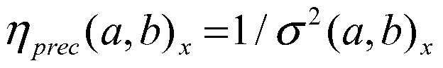
(34)

where:
<7 (α, b) χ Variance of the x-coordinate for the position fix spanning time a to b.
For example if a=b, then this is the variance of the synchronous fix. When a < b, the variance corresponds to synchronous fix at time a, that has been propagated using rover position differences, to time b.
<7 (a, b) Variance of the y-coordinate for the position fix spanning time a to b; (7 (a, b) z Variance of the z-coordinate for the position fix spanning time a to b. precis b) x Precision-based blending factor for the x-coordinate, for the position fix spanning time a to b. With analogous definitions for the y and z coordinates.
[0179] Note that the raw blending factors need to be normalized (so that they sum to 1.0).
[0180] An illustration of the precision-based blending scheme is presented in Table 10. Just the x- coordinate is included in the example. However the approach used for the y- and z-coordinate is analogous to that used for the x-coordinate.
[0181]
Epoch Factor Precision of Solution Raw Blending Normalized Blending
Indices (x-coordinate) Factors Factors
a,b
 b)x n 'precis b)x
a
1.0 1, 1 0.025 40.00 1.0
2.0 1,2 0.031 32.26 0.4363
2,2 0.024 41.67 0.5636
0 1,3 0.037 27.03 0.2735
2,3 0.030 33.33 0.3373
3,3 0.026 38.46 0.3892
0 1,4 0.043 23.26 0.1876
2,4 0.036 27.78 0.2241
3,4 0.032 31.25 0.2521
4,4 0.024 41.67 0.3361
0 1,5 0.049 20.41 0.1367
2,5 0.042 23.81 0.1595
3,5 0.038 26.31 0.1762
4,5 0.030 33.33 0.2232
5,5 0.022 45.45 0.3044
0 1,6 0.055 18.18 0.1016
2,6 0.048 20.83 0.1 164
3,6 0.042 23.81 0.1331
4,6 0.036 27.78 0.1552
5,6 0.028 35.71 0.1996
6,6 0.019 52.63 0.2941
Table 10. Precision-based blending factors for example in Table 6. The x-coordinate blending factors are computed based on the precisions of the x-coordinate shown in column 3.
[0182] Bridging Reference Station Changes
[0183] Background
[0184] In a prior invention described in GNSS Position Coasting, US Patent Publication
2010/0214162 Al {A2555}, single-difference delta phase processing is used to propagate fixed quality synchronous position results forward in time in order to bridge segments of float quality synchronous position results. The GNSS Position Coasting scheme helps to extend the amount of time that fixed quality solutions are available for high precision operation.
[0185] The use of rigorous satellite clock and orbit information for improved delta positioning is described in Vollath, Position Determination with reference data outage, US Patent No. 7,576,690. The satellite clock and orbit errors are significant component of the single -reference delta phase measurements. Once satellite clock/orbit errors are removed, the precision of the single -receiver rover position difference estimates are greatly improved.
[0186] Single -receiver delta phase processing with rigorous satellite and clock information, is termed here Precise (single-receiver) Delta Phase. When the rigorous satellite clock information is predicted in time, this is termed Predicted Precise Delta Phase.
[0187] The following events can cause interruptions to high-precision position results at the rover:
1. Switch from fixed quality to float quality synchronous position results;
2. Cycle slips occur on reference station satellite data which results in insufficient single- difference satellite tracking to perform a synchronous solution;
3. The physical reference station changes in a network data stream, which normally causes a reset in the synchronous position processor and an interruption to the position report, followed by a period of float-quality positioning.
[0188] New Approach
[0189] A new unified approach has been developed which addresses specifically issue 3 above, as well as more generally handing degraded positioning caused by issues 1,2 & 3. In the new approach, the following methods of solution propagation are used to produce the best position result (where the best result is deemed as the one with the highest precision (smallest uncertainty)):
1. Single-difference delta phase (which yields single-difference rover position difference);
2. Precise (single-receiver) delta phase (which yields precise rover position difference);
3. Predicted precise (single-receiver) delta phase (which yields predicted-precise rover position difference);
4. Single-receiver delta phase (which yields rover position difference (broadcast orbits and clocks).
[0190] FIG. 14 provides an illustration of the relative uncertainties of various solutions types over time assuming all solution types use the same satellite geometry. The axis 1205 corresponds to fixed- quality synchronous solutions, with each position 1230, identified with solid black dots. The uncertainty of the positions is represented by error bars 1235.
[0191] The float-quality synchronous positions on axis 1210, have larger uncertainty than the fixed- quality synchronous solutions, as evidenced by the longer error bars 1245. Each float-quality synchronous position, 1240, shows larger variations about the zero axis, 1210.
[0192] The error growth of single- difference rover position differences is represented by the region between the dashed lines (1255) on axis 1215. Each single- difference rover position estimate 1250, is shown by a grey circle surrounded by a black ring.
[0193] The precise single-receiver rover position difference positions are presented on axis 1220. Each position fix is marked by a black ring (1260). The error growth of the precise rover position difference estimates is shown as the region 1265, assuming that the propagation time starts at first epoch and accumulates thereafter.
[0194] The predicted-precise single-receiver rover position differences are presented on axis 1222. Each position fix is marked by a dark grey circle surrounded by a black ring (1262). The error growth of the predicted-precise rover position difference estimates is shown as the region 1267.
[0195] The single-receiver rover position differences (broadcast orbits and clocks) is shown on axis 1225, with each position fix marked by a grey ring. The error growth of the single -receiver rover position differences is defined by the region 1275.
[0196] Assuming a common satellite geometry, the time -wise error growth of single-difference rover position difference is lower than that of the precise (single -receiver) rover position difference; which is lower than the predicted-precise rover position difference; which is lower than the single -receiver rover position difference (broadcast orbits and clocks). Single-difference processing requires reference and rover receivers to be tracking common satellites. In many circumstances, the number of single- difference satellites may be less than the number of rover (single-) receiver satellites. In which case, the single-difference rover position difference error growth may be worse than that of single -receiver rover position differences. [0197] FIG. 15 presents timeline views of positions (height component only) derived from prior art and new techniques. The upper axis 1305, refers to prior-art positioning methods, while the lower axis, 1310, to new techniques. The position trace for axis 1305 is denoted 1315; for axis 1310, the position trace is denoted 1320. [0198] Considering the prior-art method (axis 1305), during times 1-2, the solution has fixed quality. Between epochs 2 & 3, there is a switch in the physical reference station (or loss of satellite tracking at the reference), this event, denoted 1325, causes the synchronous processor to reset. This results in a period of float quality synchronous positioning up until epoch 6. During the float period, the accuracy of the reported position is only decimeter-level. At epoch 6, the synchronous fixed quality is reestablished (segment 1350) and retained until reference station corrections are lost just after epoch 7. The float quality solutions are propagated using single-receiver delta positions through segment 1355.
[0199] In the new approach, precise single-receiver rover position difference processing is used at epoch 3 (denoted 1370) to propagate the fixed quality synchronous solution from epoch 2 to epoch 3. Single-difference rover position difference processing is then used at epochs 4 - 6, to produce high- quality position estimates until regular synchronous fixed quality solutions are regained at epoch 6. Precise single-receiver rover position difference processing is again used between epochs 7-9, while the reference receiver data is unavailable. Note that the use of precise-single receiver rover position difference processing and single-difference rover position differences enables fixed quality solutions to be provided (segment 1360). The rigorous clock/orbit corrections are lost at event 1335, around epoch 9, after which only single-receiver (broadcast orbits and clocks) rover position difference processing is used to deliver solutions with float quality (segment 1365).
[0200] The combination of precise single -receiver rover position difference and single-difference rover position difference processing gives the new method a clear advantage in delivering fixed quality positions, versus prior art techniques. [0201 ] FIG. 16 presents a flowchart that explains the handling of data at the rover. When new data arrives at 1505, it is tested at 1510 to see if it is rover data. If so, rover data handling occurs at 1525. Predicted Precise orbit and clock information when available (see test 1512) is handled at 1527. Test 1515 checks for the presence of Precise Orbit and Clock information. When present, the Precise Orbits and Clocks are handled at 1530. The input data is tested at 1520 to see if it is from the reference and can be single- differenced. If so, the single-difference data is handled at 1535.
[0202] FIG. 17 shows an expanded view of flowchart 1500. When rover data is received, it is used to form a rover position difference solution between the current and previous epoch (1605). The rover position difference estimate is then buffered at step 1610, and optionally used to generate a low- latency position estimate at 1612.
[0203] When available, the rigorous predicted satellite clock/orbit models are updated at 1613. The rigorous predicted clock/orbit information is optionally used at 1614 to update the rover position difference for the current data epoch. At 1615, the rigorous predicted orbit information is used to update the time sequence of rover position difference estimates. The best rover position difference time sequence is generated at 1616 based on the predicted precise rover position difference time sequence and existing broadcast rover position difference time sequence. The best rover position difference from 1616 is used to replace the predicted rover position difference time sequence at 1617. [0204] The rigorous satellite clock/orbit models are updated at 1620, as soon as rigorous orbit and clock information is received for one or more satellites. The rigorous clock models enable the rover position difference time sequence derived from broadcast clocks to be optionally refined (1625) and stored. The rigorous orbit and clock information is used to form a precise rover position difference estimate for the current and previous epochs at 1630. At step 1635, the best rover position difference time sequence is produced based on the existing precise position sequence. Finally at 1640, the predicted rover position difference time sequence is replaced by the rover position difference time sequence with the smallest error.
[0205] When synchronous reference data are received, they are used to compute single- difference delta phase measurements and rover position difference estimates at 1645. The rover position difference time sequence with the smallest uncertainty is generated at step 1650, and used to replace the existing rover position difference time sequence at 1655. A synchronous position result is produced at 1660, using the latest single-difference GNSS measurements. The best (smallest uncertainty) synchronous position solution is derived from the latest synchronous position result, and the single-difference rover position difference time sequence in step 1665. If for example the synchronous position result is float quality, then often the single-difference rover position difference time sequence that was propagated from the last fixed quality solution will be the best (smallest uncertainty). At 1670, all of the single-difference rover position differences up to the reference data time tag are replaced with the new synchronous position solution. Finally at step 1675, an optional report of the synchronous position is provided which will be latent with respect to the current time.
[0206] Following is a summary of some of the inventive concepts described herein: [0207] [Part A: Predicted precise] [TNL A-2796]
1. A positioning method, comprising:
a. obtaining GNSS data derived from signals received at a rover antenna,
b. obtaining at least one of correction data and rigorous satellite data,
c. maintaining a time sequence of at least one rover position and at least one rover
position difference with associated time tags,
d. using the time sequence to determine at least one derived rover position, e. reporting the derived rover position, and
f. maintaining a set of GNSS satellite clock error models, comprising
i. upon arrival of rover data associated with a new time tag, extending the time sequence, and
ii. upon arrival of rigorous satellite data, updating at least one clock error model.
2. The method of 1, wherein maintaining a set of GNSS satellite clock error models further comprises, upon arrival of rigorous satellite orbit and clock data, updating the time sequence.
3. The method of 1 or 2, further comprising using the updated at least one clock error model to update at least one rover position of the time sequence.
4. The method of one of 1-3, wherein the set of satellite clock error models comprises up to one clock error model per satellite.
The method of one of 1-4, wherein the correction data comprises at least one of: single-base- station observations [RTK], virtual reference station observations derived from reference stations of a regional network [VRS], synthetic base station observations derived from reference stations of a global network [SBS], synthetic reference station observations derived from reference stations of a global network with regional augmentation [SRS], and state space representations [RTCM SSR].
The method of one of 1-5, wherein rigorous satellite data comprises precise orbit and precise clock data per satellite.
Apparatus for performing a method according to one of 1-6.
A computer program comprising instructions for causing an apparatus to perform a method according to one of 1-6.
A computer program product comprising a tangible computer-readable medium embodying instructions for causing an apparatus to perform a method according to one of 1-6. [Part B: Mixed Delta - mixing quality in one epoch] [TNL A-2798] A positioning method, comprising
a. obtaining GNSS data derived from signals received at a rover antenna,
b. obtaining at least one of correction data and rigorous satellite data,
c. maintaining a time sequence of at least one rover position and at least one rover position difference with associated time tags, by estimating at least one position difference using rigorous satellite data from multiple satellites using at least two selected combinations of
i. for at least one satellite, no correction data and broadcast satellite data, ii. for at least one satellite, no correction data and rigorous predicted satellite data,
iii. for at least one satellite, no correction data rigorous satellite data for said at least one satellite,
iv. for at least one satellite, correction data and broadcast satellite data, v. for at least one satellite, rigorous predicted satellite data and correction data, vi. for at least one satellite, rigorous satellite data and correction data, d. using the time sequence to determine at least one derived rover position, and e. reporting the derived rover position.
2. The method of 1, wherein estimating at least one position difference using rigorous satellite data from multiple satellites using at least two selected combinations comprises applying a filter having two clock states per satellite.
3. The method of one of 1-2, wherein the correction data comprises at least one of: single-base- station observations [RTK], virtual reference station observations derived from reference stations of a regional network [VRS], synthetic base station observations derived from reference stations of a global network [SBS], synthetic reference station observations derived from reference stations of a global network with regional augmentation [SRS], and state space representations [RTCM SSR].
4. The method of one of 1-3, wherein rigorous satellite data comprises rigorous orbit data per satellite and rigorous clock data per satellite.
5. Apparatus for performing a method according to one of 1-4.
6. A computer program comprising instructions for causing an apparatus to perform a method according to one of 1-4.
7. A computer program product comprising a tangible computer-readable medium embodying instructions for causing an apparatus to perform a method according to one of 1-4. 9] [Part C: Improve/cleanup the buffer] [TNL A-3126]
A positioning method, comprising
a. obtaining GNSS data derived from signals received at a rover antenna,
b. obtaining at least one of correction data and rigorous satellite data,
c. maintaining a time sequence of at least one rover position and at least one rover position difference with associated time tags by,
i. upon arrival of correction data, extending the time sequence with a computed synchronized position, and
ii. upon arrival of one of correction data and rigorous satellite data, modifying at least a portion of the time sequence,
d. using the time sequence to determine at least one derived rover position, and e. reporting the derived rover position.
The method of 1, wherein the computed synchronized position comprises one of: a real-time kinematic [RTK] position, a position determined using a weighted average of integer ambiguity candidates, a position determined using a differential positioning technique
[DGPS], a position determined with the aid of an inertial navigation system, and a technique using GNSS data to determine an absolute position.
[Mixing and Replacing] The method of one of 1-2, wherein modifying at least a portion of the time sequence comprises replacing at least one position difference by at least one improved position difference [lower variance].
The method of 3, wherein replacing at least one position difference by at least one improved position difference comprises replacing at least one position difference determined using broadcast satellite data with at least one position difference determined using rigorous predicted satellite data.
The method of one of 3-4, wherein replacing at least one position difference by at least one improved position difference comprises blending at least one position difference determined using broadcast satellite data with at least one position difference determined using rigorous predicted satellite data.
The method of one of 3-5, wherein replacing at least one position difference by at least one improved position difference comprises replacing at least one position difference determined using rigorous predicted satellite data with at least one position difference determined using rigorous satellite data.
The method of one of 3-6, wherein replacing at least one position difference by at least one improved position difference comprises blending at least one position difference determined using rigorous predicted satellite data with at least one position difference determined using rigorous satellite data.
The method of one of 3-7, wherein replacing at least one position difference by at least one improved position difference comprises replacing at least one position difference determined using rigorous satellite data with at least one position difference determined using corrected single-differenced data.
The method of one of 3-8, wherein replacing at least one position difference by at least one improved position difference comprises blending at least one position difference determined using rigorous satellite data with at least one position difference determined using corrected single-differenced data.
The method of one of 3-9, wherein replacing at least one position difference by at least one improved position difference comprises replacing at least one position difference determined using corrected single-differenced data with at least one position difference determined using corrections synchronous with rover data.
The method of one of 3-10, wherein replacing at least one position difference by at least one improved position difference comprises blending at least one position difference determined using corrected single-differenced data with at least one position difference determined using corrections synchronous with rover data.
The method of one of 1-1 1, wherein maintaining a time sequence further comprises, upon arrival of rigorous satellite data, replacing at least one position difference by at least one improved position difference.
[Replacing] The method of one of 1-12, wherein modifying at least a portion of the time sequence comprises replacing a portion of the time sequence with an improved portion of the time sequence.
The method of 13, wherein the improved portion of the time sequence has an estimated precision which is better than an estimated precision of a portion of the time sequence which it replaces.
The method of one of 13-14, wherein the improved portion of the time sequence has a number of entries which is fewer than a number of entries of a portion of the time sequence which it replaces.
The method of one of 13-15, wherein the improved portion of the time sequence is determined by, starting from a position determined using corrections synchronous with rover data as an anchor position at a time tag, deriving a new anchor position for the time tag from the anchor position and at least one other previously estimated position at the time tag.
[selecting] The method of 16, wherein deriving a new anchor position for the time tag comprises selecting between the anchor position and the at least one other previously estimated position at the time tag based on comparison of an estimated precision of the anchor position with an estimated precision of the at least one other previously estimated position at the time tag.
The method of 17, wherein at least one estimated precision is determined from a covariance matrix.
The method of one of 17-18, wherein the new anchor position for the time tag is selected based on smallest estimated three-dimensional precision.
The method of one of 17-18, wherein the new anchor position for the time tag is selected based on smallest estimated horizontal precision.
The method of one of 17-18, wherein the new anchor position for the time tag is selected based on smallest vertical precision.
[blending] The method of 16, wherein deriving a new anchor position for the time tag comprises blending the anchor position with the at least one other previously estimated position at the time tag.
The method of 22, wherein blending comprises forming a weighted mean of the anchor position and at least one other previously estimated position at the time tag.
Apparatus for performing a method according to one of 1-23.
A computer program comprising instructions for causing an apparatus to perform a method according to one of 1-23.
A computer program product comprising a tangible computer-readable medium embodying instructions for causing an apparatus to perform a method according to one of 1-23. [Part D: Jump Reduction] [TNL A-2638]
A positioning method, comprising
a. obtaining for each epoch of a set of at least one epoch a respective synchronous position to be propagated to an anchor epoch,
b. for each epoch of the set, combining the respective synchronous position with at least one rover position difference defining a change of rover position from the epoch of the respective synchronous position to the anchor epoch, to obtain a respective propagated position for the anchor epoch,
c. obtaining a synchronous position for the anchor epoch,
d. blending at least one propagated position for the anchor epoch with the synchronous position for the anchor epoch to obtain a blended anchor position for the anchor epoch,
e. determining a propagated rover position for a current epoch by combining the blended anchor position with at least one rover position difference defining a change of rover position from the anchor epoch to the current epoch.
The method of 1 , wherein the blending comprises blending a selected number of propagated positions for the anchor epoch with the synchronous position for the anchor epoch.
The method of one of 1 -2, wherein the blending is based on at least one weighting factor. The method of one of 1-3, wherein at least one weighting factor is based on age of a synchronous position used to obtain a propagated position which is blended to obtain the blended anchor position for the anchor epoch.
The method of 4, wherein at least one weighting factor declines linearly with age of a synchronous position used to obtain a propagated position which is blended to obtain the blended anchor position for the anchor epoch.
The method of 4, wherein at least one weighting factor declines exponentially with age of a synchronous position used to obtain a propagated position which is blended to obtain the blended anchor position for the anchor epoch.
The method of one of 1-3, wherein at least one weighting factor is based on an estimated precision of a propagated position which is blended to obtain the blended anchor position for the anchor epoch.
The method of 8, wherein at least one weighting factor is based on an estimated precision of the synchronous position for the anchor epoch.
The method of one of 1-3, wherein the blending is proportional to respective estimated precisions of the at least one propagated position for the anchor epoch and of the synchronous position for the anchor epoch.
. Apparatus for performing a method according to one of 1-9.
. A computer program comprising instructions for causing an apparatus to perform a method according to one of 1-9.
. A computer program product comprising a tangible computer-readable medium embodying instructions for causing an apparatus to perform a method according to one of 1-9. ] [Part E: Selecting/blending] [TNL A-2797] A positioning method, comprising
a. obtaining GNSS data derived from signals received at a rover antenna,
b. obtaining correction data,
c. maintaining a time sequence of at least one rover position and at least one rover position difference with associated time tags,
d. using the time sequence to determine at least one derived rover position by, starting from a position determined using corrections synchronous with rover data as an anchor position at a time tag, deriving a new anchor position for the time tag of the anchor position and at least one other estimated rover position at the time tag of the anchor position, and
e. at least one of
i. reporting the new anchor position at the time tag as the rover position at a time associated with the time tag of the anchor position, and ii. combining the new anchor position at the time tag of the anchor position with at least one rover position difference to determine a new derived rover position for a subsequent time tag, and reporting the new derived rover position as the rover position at a time associated with the subsequent time tag.
[selecting] The method of 1, wherein deriving a new anchor position for the time tag comprises selecting between the anchor position and the at least one other previously estimated position at the time tag based on comparison of an estimated precision of the anchor position with an estimated precision of the at least one other previously estimated position at the time tag.
The method of 2, wherein at least one estimated precision is determined from a covariance matrix.
The method of one of 1-3, wherein the new anchor position for the time tag is selected based on smallest estimated three-dimensional precision.
The method of one of 1-3, wherein the new anchor position for the time tag is selected based on smallest estimated horizontal precision.
The method of one of 1-3, wherein the new anchor position for the time tag is selected based on smallest vertical precision.
[blending] The method of 1, wherein deriving a new anchor position for the time tag comprises blending the anchor position with the at least one other previously estimated position at the time tag.
The method of 7, wherein blending comprises forming a weighted mean of the anchor position and at least one other previously estimated position at the time tag.
Apparatus for performing a method according to one of 1-8.
A computer program comprising instructions for causing an apparatus to perform a method according to one of 1-8.
A computer program product comprising a tangible computer-readable medium embodying instructions for causing an apparatus to perform a method according to one of 1-8. [Part F: Correcting Delta-Phase for Incorrect Starting Position] [TNL A-2705] A positioning method, comprising
a. obtaining an approximate rover anchor position for a first epoch,
b. using the approximate rover anchor position to determine a rover position difference for at least one succeeding epoch,
c. obtaining an improved rover anchor position for the first epoch,
d. deriving an adjusted rover position difference for each said succeeding epoch, and e. deriving a rover position for a current epoch from the improved rover anchor position for the first epoch and at least one adjusted rover position difference.
2. The method of 1, wherein the approximate rover anchor position contains an initial error, wherein the rover position difference for each said succeeding epoch contains a respective partial error based on the initial error, and wherein deriving an adjusted rover position difference for each said succeeding epoch comprises correcting each rover position difference for the respective partial error.
3. Apparatus for performing a method according to one of 1-2.
4. A computer program comprising instructions for causing an apparatus to perform a method according to one of 1-2.
5. A computer program product comprising a tangible computer-readable medium embodying instructions for causing an apparatus to perform a method according to one of 1-2.
[0213] The foregoing description of embodiments is not intended as limiting the scope of but rather to provide examples of the invention as defined by the claims. Those of ordinary skill in the art will realize that the detailed description of embodiments of the present invention is illustrative only and is not intended to be in any way limiting. Other embodiments of the present invention will readily suggest themselves to such skilled persons having the benefit of this disclosure.
[0214] In the interest of clarity, not all of the routine features of the implementations described herein are shown and described. It will be appreciated that in the development of any such actual implementation, numerous implementation-specific decisions must be made to achieve the developer's specific goals, such as compliance with application- and business-related constraints, and that these specific goals will vary from one implementation to another and from one developer to another.
Moreover, it will be appreciated that such a development effort might be complex and time- consuming, but would nevertheless be a routine undertaking of engineering for those of ordinary skill in the art having the benefit of this disclosure.
[0215] In accordance with embodiments of the present invention, the components, process steps and/or data structures may be implemented using various types of operating systems (OS), computer platforms, firmware, computer programs, computer languages and/or general-purpose machines. Portions of the methods can be run as a programmed process running on processing circuitry. The processing circuitry can take the form of numerous combinations of processors and operating systems, or a stand-alone device. The processes can be implemented as instructions executed by such hardware, by hardware alone, or by any combination thereof. The software may be stored on a program storage device readable by a machine. Computational elements, such as filters and banks of filters, can be readily implemented using an object-oriented programming language such that each required filter is instantiated as needed.
[0216] Those of skill in the art will recognize that devices of a less general-purpose nature, such as hardwired devices, field programmable logic devices (FPLDs), including field programmable gate arrays (FPGAs) and complex programmable logic devices (CPLDs), application specific integrated circuits (ASICs), or the like, may also be used without departing from the scope and spirit of the inventive concepts disclosed herein.
[0217] In accordance with an embodiment of the present invention, the methods may be implemented in part on a data processing computer such as a personal computer, workstation computer, mainframe computer, or high-performance server running an operating system such as a version of Microsoft
Windows, or various versons of the Unix operating system such as Linux available from a number of vendors. The methods may also be implemented on a multiple-processor system, or in a computing environment including various peripherals such as input devices, output devices, displays, pointing devices, memories, storage devices, media interfaces for transferring data to and from the processor(s), and the like. Such a computer system or computing environment may be networked locally, or over the Internet.
[0218] Any of the above-described methods and their embodiments may be implemented in part by means of a computer program. The computer program may be loaded on an apparatus as described above. Therefore, the invention also relates to a computer program, which, when carried out on an apparatus performs portions of any one of the above above-described methods and their embodiments.
[0219] The invention also relates to a computer-readable medium or a computer-program product including the above-mentioned computer program. The computer-readable medium or computer-
program product may for instance be a magnetic tape, an optical memory disk, a magnetic disk, a magneto-optical disk, a CD ROM, a DVD, a CD, a flash memory unit or the like, wherein the computer program is permanently or temporarily stored. The invention also relates to a computer- readable medium (or to a computer-program product) having computer-executable instructions for carrying out any one of the methods of the invention.
[0220] The invention also relates to a firmware update adapted to be installed on apparatus already in the field, i.e. a computer program which is delivered to the field as a computer program product. This applies to each of the above-described methods and apparatuses.
[0221 ] Although the present invention has been described on the basis of detailed examples, the detailed examples only serve to provide the skilled person with a better understanding, and are not intended to limit the scope of the invention. The scope of the invention is much rather defined by the appended claims.
S P E C I F I C A T I O N
TITLE OF INVENTION GNSS SIGNAL PROCESSING WITH REGIONAL AUGMENTATION NETWORK
CROSS REFERENCE TO RELATED APPLICATIONS
[0001] The following are related hereto and incorporated herein in their entirety by this reference: United States Provisional Application for Patent No. 61/277,184 filed 19
September 2009 (TNL A-2585P); International Patent Application PCT/US2009/059552 filed 5 October 2009 (TNL A-2288PCT); United States Provisional Application for Patent No. 61/195,276 filed 6 October 2008 (TNL A-2288P); International Patent Application
PCT/US/2009/004471 filed 5 August 2009 (TNL A-2526PCT); International Patent Application PCT/US/2009/004473 filed 5 August 2009 (TNL A-2525PCT); International Patent Application PCT/US/2009/004474 filed 5 August 2009 (TNL A-2524PCT);
International Patent Application PCT/US/2009/004472 filed 5 August 2009 (TNL A- 2523PCT); International Patent Application PCT/US/2009/004476 filed 5 August 2009 (TNL A-2339PCT); United States Provisional Application for Patent No. 61/189,382 filed 19 August 2008 (TNL A-2339P); United States Patent Application 12/224,451 filed 26 August 2008, United States Patent Application Publication US 2009/0027625 Al (TNL A-1789US); International Patent Application PCT/US07/05874 filed 7 March 2007, International Publication No. WO 2008/008099 A2 (TNL A-1789PCT); United States Patent Application No. 11/988,763 filed 14 January 2008, United States Patent Application Publication US 2009/0224969 Al (TNL A-1743US); International Patent Application No.
PCT/US/2006/034433 filed 5 September 2006, International Publication No. WO
2007/032947 Al (TNL A-1743PCT); United States Patent No. 7,432,853 granted 7 October 2008; (TNL A-1403US); (TNL A-1403PCT); International Patent Application No.
PCT/US2004/035263 filed 22 October 2004 and International Publication Number WO 2005/045463 Al (TNL A-1403PCT; United States Patent No. 6,862,526 granted 1 March 2005 (TNL A-1006US); and United States Provisional Application for Patent No. 61/396,676, filed 30 May 2010 (TNL A-2751P).
TECHNICAL FIELD
[0002] The present invention relates to the field of Global Navigation Satellite Systems GNSS). More particularly, the present invention relates to methods and apparatus for processing of GNSS data with regional augmentation for enhanced precise point positioning.
BACKGROUND ART
[0003] Global Navigation Satellite Systems (GNSS) include the Global Positioning System (GPS), the Glonass system, the proposed Galileo system, the proposed Compass system, and others. Each GPS satellite transmits continuously using two radio frequencies in the L-band, referred to as LI and L2, at respective frequencies of 1575.41 MHz and 1227.60 MHz. Two signals are transmitted on LI, one for civil users and the other for users authorized by the United States Department of Defense (DoD). One signal is transmitted on L2, intended only for DoD-authorized users. Each GPS signal has a carrier at the LI and L2 frequency, a pseudo-random number (PRN) code, and satellite navigation data. Two different PRN codes are transmitted by each satellite: a coarse acquisition (C/A) code and a precision (P/Y) code which is encrypted for DoD-authorized users. Each C/A code is a unique sequence of 1023 bits, which is repeated each millisecond. Other GNSS systems likewise have satellites which transmit multiple signals on multiple carrier frequencies.
[0004] FIG. 1 schematically illustrates a typical prior-art scenario to determine the position of a mobile receiver (rover). Rover 100 receives GPS signals from any number of satellites in view, such as SVl, SV2, and SVM, shown respectively at 110, 120 and 130. The signals pass through the earth's ionosphere 140 and through the earth's troposphere 150. Each signal has two frequencies, LI and L2. Receiver 100 determines from the signals respective pseudo- ranges, PR1, PR2, PRM, to each of the satellites. Pseudo-range determinations are distorted by variations in the signal paths which result from passage of the signals through the ionosphere 140 and the troposphere 150, and from multipath effects, as indicated schematically at 160.
[0005] Pseudo-range can be determined using the C/A code with an error of about one meter, a civil receiver not using the military-only P/Y code determines rover position with an error in the range of meters. However, the phases of the LI and L2 carriers can be measured with an accuracy of 0.01 - 0.05 cycles (corresponding to pseudo-range errors of 2 mm to 1 cm), allowing relative position of the rover to be estimated with errors in the range of millimeters
to centimeters. Accurately measuring the phase of the LI and L2 carriers requires a good knowledge of the effect of the ionosphere and the troposphere for all observation times.
[0006] Relative positioning allows common-mode errors to be mitigated by differencing the observations of the rover with observations of a reference station at a known location near the rover, e.g., within 50-100 km. The reference station observations can be collected at a physical base station or estimated from observations of a network of reference stations. See for example U.S. Pat. No. 5,477,458 "Network for Carrier Phase Differential GPS
Corrections" and U.S. Pat. No. 5,899,957 "Carrier Phase Differential GPS Corrections Network."
[0007] Precise point positioning (PPP), also called absolute positioning, uses a single GNSS receiver together with precise satellite orbit and clock data to reduce satellite -related error sources. A dual-frequency receiver can remove the first-order effect of the ionosphere for position solutions of centimeters to decimeters. The utility of PPP is limited by the need to wait longer than desired for the float position solution to converge to centimeter accuracy. And unlike relative positioning techniques in which common-mode errors are eliminated by differencing of observations, PPP processing uses undifferenced carrier-phase observations so that the ambiguity terms are corrupted by satellite and receiver phase biases. Methods have been proposed for integer ambiguity resolution in PPP processing. See, for example, Y. Gao et al., GNSS Solutions: Precise Point Positioning and Its Challenges, Inside GNSS, November/December 2006, pp. 16-18. See also United States Provisional Application for Patent No. 61/277,184 filed 19 September 2009 (TNL A-2585P).
[0008] Improved GNSS processing methods and apparatus are desired, especially to achieve faster convergence to a solution, improved accuracy and/or greater availability.
SUMMARY
[0009] Improved methods and apparatus for processing of GNSS data with augmentation for enhanced precise positioning are presented.
[0010] Some embodiments of the invention provide methods and/or apparatus for processing of GNSS data derived from multi- frequency code and carrier observations are presented which make available correction data for use by a rover located within the region, the correction data comprising: the ionospheric delay over the region, the tropospheric delay over the region, the phase-leveled geometric correction per satellite, and the at least one code bias per satellite.
[0011] Some embodiments provide methods and apparatus for determining a precise position of a rover located within a region in which a GNSS receiver is operated to obtain multi- frequency code and carrier observations and correction data, to create rover corrections from the correction data, and to determine a precise rover position using the rover observations and the rover corrections.
[0012] In some embodiments the correction data comprises at least one code bias per satellite, a fixed-nature MW bias per satellite and/or values from which a fixed-nature MW bias per satellite is derivable, and an ionospheric delay per satellite for each of multiple regional network stations and/or non-ionospheric corrections.
[0013] In some embodiments the correction data comprises at least one code bias per satellite, a fixed-nature MW bias per satellite and/or values from which a fixed-nature MW bias per satellite is derivable, and an ionospheric delay per satellite for each of multiple regional network stations and an ionospheric phase bias per satellite, and/or non-ionospheric corrections.
[0014] Some embodiments provide methods and apparatus for encoding and decoding the correction messages containing correction data in which network messages include network elements related to substantially all stations of the network and cluster messages include cluster elements related to subsets of the network.
[0015] Some embodiments provide regional correction data streams prepared in accordance with the methods and suitable for broadcast and use by mobile GNSS receivers within a network area.
[0016] Some embodiments provide computer program products embodying instructions for carrying out the methods.
BRIEF DESCRIPTION OF DRAWING FIGURES
[0017] These and other aspects and features of the present invention will be more readily understood from the embodiments described below with reference to the drawings, in which:
FIG. 1 schematically illustrates a typical prior-art scenario to determine a rover position;
FIG. 2 schematically illustrates a system in accordance with some embodiments of the invention;
FIG. 3 schematically illustrates a global network processor in accordance with some embodiments of the invention;
FIG. 4 schematically illustrates a regional network processor in accordance with some embodiments of the invention;
FIG. 5 schematically illustrates a regional network process in accordance with some embodiments of the invention;
FIG. 6 schematically illustrates augmented precise point positioning in accordance with some embodiments of the invention;
FIG. 7 schematically illustrates generating synthetic reference station data for augmented precise point positioning in accordance with some embodiments of the invention;
FIG. 8 schematically illustrates augmented precise point positioning with differential processing in accordance with some embodiments of the invention;
FIG. 9 schematically illustrates augmented precise point positioning with differential processing in accordance with some embodiments of the invention;
FIG. 10 schematically illustrates augmented precise point positioning with differential processing accordance with some embodiments of the invention;
FIG. 11 schematically illustrates construction of synthetic reference station observations in accordance with some embodiments of the invention;
FIG. 12 schematically illustrates an ionospheric shell and a portion of a tropospheric shell surrounding the Earth;
FIG. 13 illustrates a slanted ray path from a satellite to a receiver passing through the troposphere;
FIG. 14 illustrate the relation between Total Electron Content along a slant path and Vertical Total Electron content;
FIG. 15 illustrates how ionosphere parameters describe the ionosphere at a piercepoint relative to a reference point;
FIG. 16 schematically illustrates troposcaling in accordance with some embodiments of the invention;
FIG. 17 schematically illustrates spacing of locations for geometric correction terms are determined in accordance with some embodiments of the invention;
FIG. 18 schematically illustrates a linear model for determining the geometric correction at a rover location from geometric corrections three arbitrary locations in accordance with some embodiments of the invention;
FIG. 19 schematically illustrates ionospheric delay IPBS at a physical base station location PBS and ionospheric delay ISRS at a synthetic reference station location SRS;
FIG. 20 schematically illustrates regional correction message encoding in accordance with some embodiments of the invention;
FIG. 21 schematically illustrates clusters of regional network stations in accordance with some embodiments of the invention;
FIG. 22 shows an example of a rover located within a regional network having clusters in accordance with some embodiments of the invention;
FIG. 23 is a schematic diagram of a computer system in accordance with some embodiments of the invention; and
FIG. 24 is a schematic diagram of a GNSS receiver system in accordance with some embodiments of the invention;
DETAILED DESCRIPTION
Part i: Introduction
[0018] Methods and apparatus in accordance with some embodiments involve making available and/or using correction data with rover observations of GNSS satellite signals for precise navigation or positioning of a rover located within a region. The correction data comprises (1) at least one code bias per satellite, i.e. a fixed-nature MW bias per satellite (or values from which a fixed-nature MW bias per satellite is derivable), (2) a phase-leveled geometric correction per satellite derived from the network fixed double difference ambiguities, and (3) an ionospheric delay per satellite for each of multiple regional network stations, and optionally an ionospheric phase bias per satellite, and/or non-ionospheric corrections.
[0019] The corrections are determined at least in part from code and carrier phase observations of GNSS satellite signals by reference stations of a network distributed over the region. The code bias is derived from fixed ambiguities (e.g., double-differenced) of the regional reference station network.
[0020] The corrections enable reconstruction of code and phase observations of the reference stations. The ability to reconstruct the geometric part (ionospheric-free observation combinations) is based on the phase-leveled geometric correction term per satellite. This geometric correction term encapsulates the integer nature of the ambiguity and compensates the orbit error and satellite clock error seen in the regional reference station network.
[0021] If m stations of the regional network observe n satellites, the transmission bandwidth needed to transmit m x n observations and m x n carrier observations on each GNSS frequency would be impractical. Some embodiments of the invention substantially reduce this bandwidth requirement. Only one or three geometric corrections is/are transmitted for each of the n satellites in accordance with some embodiments. Only one code bias is transmitted for each of the n satellites in accordance with some embodiments. Only one tropospheric value is optionally transmitted for each of the m stations. The non-ionospheric part of the regional network correction comprises the code biases, phase-leveled geometric correction and the optional tropospheric values.
[0022] In some embodiments, the ionospheric part of the regional reference station network correction is based on observation space. It is derived from the ionospheric carrier-phase dual-frequency combination minus the ambiguity determined from processing the regional
network observations. Thus m x n ionospheric corrections are optionally transmitted for processing of rover observations.
[0023] In some embodiments, an absolute ionosphere model estimated from the network, or a global/regional ionosphere model like WAAS, IONEX or GAIM is used; an ionospheric phase bias per satellite and per station is derived together with the ionospheric correction per satellite per station. Thus m x n ionospheric corrections plus n ionospheric phase biases are optionally transmitted for processing of rover observations. Carrier phase observations of the regional network's reference stations (e.g., on carriers LI and L2) can be fully reconstructed using the geometric part (phase-leveled geometric correction and tropospheric corrections) together with the ionospheric part (ionospheric corrections and optional ionospheric phase biases). If the optional tropospheric corrections are not provided, the tropospheric delay at the rover can be estimated in rover processing, at the cost of slower convergence.
[0024] Double differencing of the reconstructed observations of the regional network stations with raw LI and L2 carrier-phase observations of the rover receiver results in ambiguity values which are close to integer.
[0025] Some advantages of this approach are:
O No master station is required. This leads to a simpler algorithm for generating
synthetic reference station data and reduced burden for encoding and decoding the correction messages when these are transmitted for processing of rover observations.
O Multipath mitigation and noise reduction. The phase-leveled geometric correction term per satellite is generated using all stations in the regional reference station network. Reconstructed observations thus mitigate the multipath of all stations, instead of the inherent mitigation of the full multipath and noise of a master station. In addition, the ionospheric part is in some embodiments smoothed over time by the regional network processor to reduce noise.
O Smooth transition from only global network corrections to global corrections
augmented with regional corrections when the rover moves into a region covered by a regional network. The regional corrections add a geometric correction per satellite together with ionospheric and/or non-ionospheric corrections. When a rover moves into a region covered by a regional network, processing of the rover observations benefits immediately from the added regional corrections.
O Bandwidth reduction. With a regional network of, for example, 80 reference stations tracking 12 satellites, a transmission bandwidth of about 2200-2500 bits/second should provide an update rate of 10 seconds even without optimizations (described
below) that become possible because of the changed information content of the messages.
Part 2: Reconstructing Code and Carrier-Phase Observations
Part 2.1 Carrier-Phase Observation Data with Fixed Double-Difference
Ambiguities
[0026] GPS Li and L2 carrier phase observations can be expressed as:
Lx= <px = p + T + Il+c-(tr -ts) + b[ -b + λιΝι+νι (1) p + T + ^Il+c-{tr-ts) + b2 r-bs 1 + 2N2+v2 (2) where
Lj and L2 are the Li and L2 carrier phase observations in metric units,
<p2 are the Li and L2 carrier phase observations in cycles,
P is the geometric range between antenna phase centers of satellite and receiver,
T is the tropospheric delay,
is the Li ionospheric delay,
i*and tr are the satellite clock error and receiver clock error, respectively, 0j Sand b2 are the satellite Li phase bias and satellite L2 phase bias, respectively, b and b2 are the receiver Li phase bias and satellite L2 phase bias, respectively, Nj and N2 are "true" Li and L2 integer ambiguities, respectively, and jand v2 are phase noise plus multipath of Li and L2, respectively.
ospheric-free carrier-phase observation can be expressed as
L1F =p + T + c-(tr-0 + b -bc°+Nc +uc (3)

is the ionospheric-free ambiguity,

are respectively the receiver and satellite ionospheric-free satellite phase biases, and
Nw = N, - N2 . (6) is the widelane ambiguity .
[0028] The ionospheric phase observation Ln mapped to frequency LI can be written as
Al - A2
(7)
where

(8)
is the ionospheric ambiguity, and
(9)
are respectively the receiver and satellite ionospheric phase biases.
[0029] The formulas are simplified by forming the single difference of observations of two satellites at each reference station to cancel out receiver clock error and receiver phase bias. The single-difference LI and L2 carrier -phase combinations are

The single difference ionospheric -free phase is then expressed as (12)

[0030] Assuming the single difference integer ambiguities estimated by the network processor are VNW, VN2 , the estimated single-difference ionospheric-free satellite phase bias Vb can be derived as
Vbc s = VLc - Vp - VT + cVt > - VNW + - ^- VN2 ) (is) where
V 5 is the single difference geometric range computed from the ephemeris,
V? s is the single difference satellite clock error computed from the ephemeris, and
VT is the single difference tropospheric delay estimated in the network processor.
[0031] If the satellite orbits and clocks are perfect and the tropospheric delays estimated from the network are also perfect, and ignoring the phase noise, the relationship of the derived single-difference ionospheric-free satellite phase bias to the "true" bias VZ>? is

[0032] The derived single-difference ionospheric-free satellite phase bias is offset by a linear combination of integer widelane and L2 cycles if the fixed ambiguities are not equal to the "true" ambiguities. If the double difference ambiguities between all the reference stations are fixed correctly, this equation is valid for all the stations
[0033] A network-derived ionospheric-free phase bias per satellite is generated by combining the ionospheric-free biases derived from all stations (for example, by averaging or least squares). In reality, the orbit, clock computed from ephemeris and estimated tropospheric delay are not perfect, all the common errors mapped to line of sight from receiver to satellite are absorbed by this satellite bias term. As this term preserves the integer nature of phase observations and purely geometric correction, this term is also called a phase-leveled geometric correction.
[0034] The single difference ionospheric phase observation can be expressed as
VLn = V/1 + VZ> -- -VNw + -^-VN2 + VVl . (15)
[0035] Ignoring the phase noise and assuming the satellite bias cannot be separated from the ionospheric delay, with the network derived single difference ambiguities the derived LI ionospheric delay is expressed as:
V/, = VLn + ( ^ 7 VNW 4— VN2)
= VIl + Vb - -^ (VNw - VN + -^ (VN2 - VN2) . (16)
A — Ay Ay + Aj
= V/, + Vb;— VdNw + ^^VdN2
Aj— Α^ + Aj
This is not the "true" ionospheric delay, but is biased by a combination of integer widelane . L2 cycles and an ionospheric phase bias.
[0036] Alternatively, if the absolute ionosphere model is estimated with the network data (for example as described in United States Provisional Application for Patent No. 61/396,676, filed 30 May 2010, Attorney Docket TNL A-2751P, the content of which is incorporated herein by this reference), or a global ionosphere model is available (for example WAAS, GAIM, or IONEX), by using Eq (15), the satellite ionosphere bias can be estimated with a least squares filter or Kalman filter. To avoid rank deficiency, one satellite bias can be set to zero, or a zero mean constraint (the sum of all satellite biases equal to zero) can be used.
[0037] The LI ionospheric delay can be expressed as:
VJ, = VLn - Vb + (- -VNW --A- VN2 ) (16a)
A — Ay Ay + A
Where V6 is the estimated single difference ionospheric phase bias.
[0038] The main difference between Eq (16) and Eq (16a) is that, in Eq (16a), the single- differenced ionospheric satellite phase bias V6 is estimated with an ionosphere model and excluded from single-differenced ionospheric correction, while in Eq (16) the single-differenced ionospheric satellite phase bias Vbj is inherently included in the ionospheric delay.
[0039] In principle, with Eq (16), it is not necessary to estimate an ionosphere model over the network as far as the network ambiguities can be fixed, i.e., with the MW combination to fix widelane ambiguities and ionospheric- free phase combination to fix narrowlane ambiguities. An advantage of this approach is that the system is insensitive to the activity of ionosphere. A disadvantage is that the derived ionospheric correction is not bias free. For satellite- to-satellite single-differenced ionospheric correction, it contains the single-differenced satellite ionospheric phase bias. For undifferenced ionospheric correction, it contains a satellite ionospheric
phase bias and a receiver ionospheric phase bias. So the ionospheric correction generated with Eq (16) is only consistent in double difference. This means the computation of the ionospheric correction at a Synthetic Reference Station (SRS) location has to be done in differential way — difference between the SRS location and a nearby physical reference station (termed a Physical Base Station, or PBS) and then add to the ionospheric correction from one of the physical reference stations. This implies that the SRS data cannot be generated for a satellite for which ambiguities are not fixed at the PBS. If there are only a few satellites in view at the SRS location or the satellite geometry is bad, this could lead to large positioning error for the rover.
[0040] In contrast, the ionospheric correction generated with Eq (16a) is consistent with the used absolute ionosphere model. By estimating the satellite/receiver ionospheric phase bias, the derived ionospheric corrections are consistent in undifferenced mode, so the generation of ionospheric correction at the SRS location does not rely on any physical reference station. Insofar as ambiguities are fixed for a satellite at some reference stations, the ionospheric correction can be generated for the SRS location. When used with the ionospheric-free correction per satellite, the generated SRS data is fully synthetic.
[0041] With derived single difference ionospheric-free satellite phase bias and ionospheric delay/ionospheric satellite phase bias, LI and L2 phase observations can be fully reconstructed. The reconstructed sin le difference LI carrier phase is

= Vp + VT - cV + VIX + V6 + λχ (VdNw + VdN2 )
= Vp + VT - cVf + VIX + Vb[ + xVdNx
and the reconstructed single difference L2 carrier phase is

= Vp + VT - cVt* + -^VIl + Vb2 + 2VdN2
Comparing Eq. (17) and Eq. (18) with Eq. (l O) and Eq. (11), it can be seen that the reconstructed single difference LI and L2 phases are the original phases plus an offset of integer ambiguity.
[0042] The formulas above are derived in satellite-to-satellite single differences. These apply to non-differenced observations if a receiver-dependent bias is added to each satellite observed at the reference station. The receiver bias term is absorbed by the receiver clock term.
[0043] Tropospheric delay is estimated in the regional network using zenith total delay (ZTD) per station or a troposcaling factor per station and using a standard tropospheric model (e.g. Neill, Hopfield, etc.) and a mapping function to map a tropospheric delay for line of sight from each reference station to each satellite, in some embodiments. The a priori tropospheric model used at the regional network processor is the same as that used in processing of rover observations in some embodiments.
[0044] The relation between the estimated tropospheric delay to estimated zenith total delay and troposcaling can be written as:
T = ZTD - MP = (1 + Ts ) -ZTDmoielMP (19) where:
T is the tropospheric delay of a given satellite at a reference station,
ZTD is the estimated tropospheric zenith total delay at the reference station, MP is the mapping function of the a priori troposphere model used in the network processor,
is the troposcaling factor, and
ZTD, mode/ is the zenith total delay computed from the a priori troposphere model.
Part 2.2 Reconstructing LI and L2 Pseudorange Observations
[0045] For the narrow-lane pseudorange combination/^ , narrow-lane code biases (derived, for example, from a global network) are applied to obtain integer nature wide-lane carrier phase ambiguities using wide-lane carrier minus narrow-lane code filters; this is also known as the Melbourne-Wiibbena (MW) widelaning technique.
[0046] The constructed narrow-lane code combinations are bias free in the sense of a geometric pseudorange measurement if the MW code bias is estimated in the regional network processor. If the MW code bias is derived from another source (e.g., a global network) and applied in the regional network processor to determine widelane ambiguities, the constructed narrow-lane codes are also bias free. While it is not required that the narrowlane code be bias free, in some embodiments it is bias free.
[0047] The single difference narrowlane code and widelane phase can be written, respectively, as
VPN = Vp + VT - cV + ^ V/, + VBN + νεΝ , (20)
(Λ ~ A\)
A2
VLW = λ„φν = Vp + VT - cV + 2 VI, + Vbw + ^NW + Vvw . (21)
(Λ - )
-Wiibbena combination is given by

where VBNW is the MW code bias derived, for example, by the global network processor.
This MW code bias term BNW is a combination of code bias and carrier-phase bias and is used when fixing the widelane ambiguity in the network processing.
[0049] Narrowlane code observations and ionospheric-free code observations can be reconstructed respectively as
VPN = VLC + Λ VA + VZW (23)
A2 - Al )
VPIF = VLIF (24)
[0050] Finally, LI code observations and L2 code observations can be reconstructed respectively as
= VLIF - V/j + aVB^ (25)
VP2 = VLIF - -2- V/, + (NB^ (26) where a—— and β—— .
By using these two factors, the MW code bias term is cancelled out in the ionospheric-free code combination and is only present in narrowlane code combination.
[0051] In summary, the regional network processor generates correction terms comprising a code bias per satellite and at least one of an ionospheric delay per satellite and a non- ionospheric correction. They may include:
o A satellite-dependent bias term per satellite derived from the network fixed double
difference ambiguities. This bias term encapsulates the integer nature of the ambiguities and compensates the orbit error and satellite clock error seen in the regional reference station network (Eq. 13).
O A tropospheric zenith total delay per station or troposcaling per station (Eq.19).
O An ionospheric correction per station per satellite (Eq. 16) or, alternatively, an
ionospheric correction per station per satellite plus an ionospheric phase bias per satellite Eq.(16a).
O An MW code bias term. This term can be derived from a global network processor or regional network (Eq.22). For an explanation of the satellite dependent bias term, also called "uncalibrated phase delays" ("UPD"), see Ge et al., "Resolution of GPS carrier- phase ambiguities in Precise Point Positioning (PPP) with daily observations," Journal of Geodesy, Vol. 82, No. 7, July 2008, pages 401-412.
[0052] Code observations and carrier-phase observations of each reference station in the regional network can be reconstructed using these corrections.
Part 2.3 Constructing Synthetic Reference Station Data for Processing of Rover
Observations
[0053] The construction of synthetic reference station (SRS) data is similar to the reconstruction of pseudorange and carrier phase data at a reference station described in Part 2.2 above, except that the tropospheric delays are derived (or interpolated) from the troposcaling (zenith total delay) corrections and the and the ionosphere delays are derived (or interpolated) from the ionospheric corrections supplied by the regional network.
[0054] For example, constructed observations for an SRS location within the region of the regional network are given by
™ = = (PSRS - et * + IlSKS + TSRS , (27)
- λ2
L2sRS = *τ 2αα = (pSRS - ct s + bc s) + -f- /, + TSRS , (28) TSRs = (TSSRS + i ZTDmoielsRs - MP , (29) where:
L, is the constructed SRS LI carrier-phase observation in metric units,
L is the constructed SRS L2 carrier-phase observation in metric units,
φλ is the constructed SRS LI carrier-phase observation in cycles,
2 is the constructed SRS L2 carrier-phase observation in cycles,
pSRS is the geometric range from the selected (SRS) location to the satellite computed from ephemeris (precise orbits 350 and clocks 375 from global network processor, or IGU URO; or broadcast orbits and clocks from satellite navigation message or any other source of orbits and clock with enough accuracy to correctly fix ambiguities in the regional network processor; the required accuracy depends on the size of the regional network),
t s is the satellite clock error computed from ephemeris,
0 is the phase-leveled geometric correction derived from the network processing,
IlSRS is the ionospheric correction mapped to GPS LI frequency for the selected (SRS) location,
TSRS is the tropospheric correction for the selected (SRS) location, and
TSSRS is the troposcaling for the selected (SRS) location from regional network troposcaling estimation.
[0055] Synthetic reference station (SRS) observations are in some embodiments generated in an SRS module. The SRS module can be situated at the regional network processor (at the "server side," e.g., in a server computer), at the rover (at the "rover side," e.g., in the rover processor or in a client computer associated with the rover), or at any other suitable location.
[0056] If the SRS observations are generated at the regional network processor, the ephemeris used to generate SRS corrections can be exactly the same as the one used in the network processing, b can be used directly to generate SRS observations.
[0057] However, if the SRS observations are generated on the rover side, transmission latency and data corruption via the communication link from network processor to rover side processor may make it impractical or impossible to assure the same ephemeris is used unless a complicated validation algorithm is implemented. Instead, in some embodiments a
geometric correction which contains geometric range for an arbitrary location combined with (minus) satellite clock error and (plus) satellite bias is transmitted. This geometric correction term carries over to the rover side the orbit and clock used on the server side, avoiding the need to maintain consistency of orbit and clock between server side and rover side.
[0058] In addition, if this geometric correction term is transmitted for three arbitrary locations (e.g., within the region of the regional network), a linear model can be used to compensate the satellite orbit error for other locations (e.g., the selected SRS location which may be a rover location known only with low accuracy). A linear model is suitable for this purpose because the orbit error mapped to line of sight is very linear over a local region.
[0059] The corrected geometric range computed for a given location i is written as:
Gt = pt - c t ° + b; (30) where
pt is the geometric range computed from server ephemeris,
t s is the satellite clock error, and
0 is ionospheric-free carrier phase satellite bias derived from the network processing.
[0060] Geometric range pi and satellite clock error Is can be computed (e.g., at the rover) for the same location using the satellite's broadcast navigation message (broadcast ephemeris). The geometric range difference dpt between the geometric range p computed from broadcast ephemeris adjusted for broadcast satellite clock error r and the geometric correction Gt from the regional network for the same location is
dpt = (pt - cP) - Gt . (31)
[0061] With geometric range correction values drt for three locations in the network region, a linear model is used in some embodiments to calculate a geometric range correction dpSRS for a selected (SRS) location within the network region. The corrected geometric range for the selected (SRS) location is then
GSRS = (PsRS - - dPsRS (32) where
pSRS is the geometric range from satellite to the selected (SRS) location determined from the broadcast ephemeris,
t s is the satellite clock error determined from the broadcast ephemeris, and dpSRS is the geometric range correction for the selected (SRS) location.
[0062] In this case, the rover does not require precise orbit and clock; broadcast orbit and clock information is sufficient. Spacing between the three arbitrary locations should be large enough and with good geometry to minimize the error of building the linear model.
[0063] In some embodiments the geometric bias per satellite is transmitted to the SRS module (e.g., at the rover) for each epoch of synthetic reference station data to be generated. Eq. (27) and Eq. (28) can be rewritten respectively for the SRS location as
(33)
■■λ2φ2 r + L T (34)
[0064] Troposcaling and ionospheric correction for the selected (SRS) location are computed for example using interpolation, least squares adjustment with the troposcaling, and ionospheric correction from the reference stations. While the coordinates of the reference stations are used in troposcaling and residual interpolation, a resolution of 10m to 100m is sufficient for this purpose.
[0065] A method used in some embodiments is the WLIM (Weighted Linear Interpolation Method), in which a linear model centered at SRS location is computed using least square adjustment with the corrections from at least three reference stations.

where
(i—l,2...n) are troposcaling values at each of n reference stations, or ionospheric
correction of a satellite (or satellite to satellite difference of observations at a reference station) for each of n reference stations,
AN, , AE T are the north and east coordinate differences, respectively, from the selected
(SRS) location to the reference stations, and
a, b, c are estimates for constant part, north and east gradient.
[0066] Using least squares adjustment gives an estimate X where
X = (AT PA)'1 AT PR (36) where
is a distance-dependent weighting matrix,
and a corresponding variance of unit weight: cr0 where
VTPV
(37)
and a covariance matrix Q for X:
Q = a0 2 - (ATPA)-1 . (38)
[0067] In some embodiments, the troposcaling correction for a selected (SRS) location is obtained by taking the constant part from the model, because the model is centered at the SRS location. For ionospheric correction, this method is applicable only when the ionospheric delay per satellite / per station is computed with Eq(16a).
[0068] In some embodiments, the troposcaling correction and/or ionospheric correction for a selected (SRS) location is/are obtained by taking the difference between the SRS location and the nearest reference station to the SRS location, and adding the respective
troposcaling/ionospheric correction of that reference station
rSRS = BX + rx and aS 2 RS = BQBT (39) where
B— [θ AN AE and AN, AE are the respective north coordinate difference and east coordinate difference between the SRS and nearest reference station to SRS location, and
Tj is the troposcaling/ionospheric correction respectively of the nearest reference station.
Part 3: System Overview
[0069] FIG. 2 schematically illustrates a system 200 in accordance with some embodiments of the invention. Reference stations of a global (worldwide) tracking network, such as reference stations 205, 210, ...215, are distributed about the Earth with the aim of having substantially continuous observability of most or all GNSS satellites. The position of each reference station is known very precisely, e.g., within less than 2 cm. Each reference station is equipped with an antenna and tracks the GNSS signals transmitted by the satellites in view at that station, such as GNS satellites 220, 225, ... 230. The GNSS signals have codes modulated on each of two or more carrier frequencies. Each reference station of the global network acquires GNSS data 305 representing, for each satellite in view at each epoch, carrier-phase (carrier) observations of at least two carriers, and pseudorange (code) observations of the respective codes modulated on at least two carriers. The reference stations also obtain the broadcast navigation message with almanac and ephemerides of the satellites from the satellite signals. The almanac contains the rough position of all satellites of the GNSS, while the so-called broadcast ephemerides provide more precise predictions (ca. 1 m) of the satellites' positions and the satellites' clock error (ca. 1.5 m) over specific time intervals.
[0070] GNSS data collected at the reference stations of the global network are transmitted via communications channels 235 to a global network processor 240. Global network processor 240 uses the GNSS data from the reference stations of the global network with other information to generate a global correction message containing precise satellite position and clock data, as described for example in United States Provisional Application for Patent
No. 61/277,184 filed 19 September 2009 (TNL A-2585P). The global correction message is transmitted for use by any number of GNSS rover receivers. The global correction message is transmitted for example as shown in FIG. 2 via communications channel/s 245 and an uplink 250 and a communications satellite 255 for broadcast over a wide area; any other suitable transmission medium may be used including but not limited to radio broadcast or mobile telephone link. Rover 260 is an example of a GNSS rover receiver having a GNSS antenna 265 for receiving and tracking the signals of GNSS satellites in view at its location, and optionally having a communications antenna 270. Depending on the transmission band of the global correction message, it can be received by rover 260 via GNSS antenna 265 or communications antenna 270. The system of FIG. 1 as described thus far is as described in
United States Provisional Application for Patent No. 61/277,184 filed 19 September 2009 (TNL A-2585P).
[0071] FIG. 2 shows additional elements of a system in accordance with embodiments of the present invention. Reference stations of a regional (local) tracking network, such as reference stations 280, 282, ... 284, are distributed within a region of the Earth with the aim of observing GNSS satellites when they are visible over the region. The position of each reference station is known very precisely, e.g., within less than 2 cm. Each reference station is equipped with an antenna and tracks the GNSS signals transmitted by the satellites in view at that station, such as GNS satellites 220, 225, ... 230. Each reference station of the regional network acquires GNSS data representing, for each satellite in view at each epoch, carrier- phase (carrier) observations of at least two carriers, and pseudorange (code) observations of the respective codes modulated on at least two carriers. The regional reference stations typically also obtain the broadcast navigation message with almanac and ephemerides of the satellites from the satellite signals.
[0072] GNSS data collected at the reference stations of the regional network are transmitted via communications channels 288 to a regional network processor 290. Regional network processor 290 uses the GNSS data from the reference stations of the regional network with other information to generate a regional correction message containing correction data as described below. The regional correction message is transmitted for use by any number of GNSS rover receivers within the region of the regional network. The regional correction message is transmitted for example as shown in FIG. 2 via communications channel/s 292 and
an uplink such as uplink 250 and a communications satellite 255; any other suitable transmission medium may be used including but not limited to radio broadcast or mobile telephone link. The regional correction message can also be transmitted using an uplink and/or communications satellite other than those used for the global network message.
Part 3: Global Network Corrections
[0073] FIG. 3 is a schematic diagram showing principal components of the process flow 300 of a global network processor 240. Detailed description is provided in United States Provisional Application for Patent No. 61/277,184 filed 19 September 2009 (TNL A-2585P). Data from the global network of reference stations are supplied without corrections as GNSS data 305 or after correction by an optional data corrector 310 as corrected GNSS data 315, to four processors: a code clock processor 320, a Melbourne-Wiibbena (MW) bias processor 325, an orbit processor 330, and a phase clock processor 335.
[0074] Data corrector 310 optionally analyzes the raw GNSS data 305 from each reference station to check for quality of the received observations and, where possible, to correct the data for cycle slips, which are jumps in the carrier-phase observations occurring, e.g., each time the receiver has a loss of lock. Commercially-available reference stations typically detect cycle slips and flag the data accordingly. Cycle slip detection and correction techniques are summarized, for example, in G. Seeber, SATELLITE GEODESY, 2nd Ed. (2003) at pages 277-281. Data corrector 310 optionally applies other corrections. Though not all corrections are needed for all the processors, they do no harm if applied to the data. For example as described below some processors use a linear combination of code and carrier observations in which some uncorrected errors are canceled in forming the combinations.
[0075] Observations are acquired epoch by epoch at each reference station and transmitted with time tags to the global network processor 240. For some stations the observations arrive delayed. This delay can range between milliseconds and minutes. Therefore an optional synchronizer 318 collects the data of the corrected reference station data within a predefined time span and passes the observations for each epoch as a set to the processor. This allows data arriving with a reasonable delay to be included in an epoch of data.
[0076] The MW bias processor 325 takes either uncorrected GNSS data 305 or corrected GNSS data 315 as input, since it uses the Melbourne-Wiibbena linear combination which cancels out all but the ambiguities and the biases of the phase and code observations. Thus only receiver and satellite antenna corrections are important for the widelane processor 325. Based on this linear combination, one MW bias per satellite and one widelane ambiguity per receiver-satellite pairing are computed. The biases are smooth (not noisy) and exhibit only some sub-daily low-rate variations. The widelane ambiguities are constant and can be used as
long as no cycle slip occurs in the observations on the respective satellite -receiver link. Thus the bias estimation is not very time critical and can be run, e.g., with a 15 minute update rate. This is advantageous because the computation time grows with the third power of the number of stations and satellites. As an example, the computation time for a global network with 80 stations can be about 15 seconds. The values of fixed widelane ambiguities 340 and/or widelane biases 345 are optionally used in the orbit processor 330 and/or the phase clock processor 335, and/or are supplied to a scheduler 355. MW bias processor 325 is described in detail in Part 7 of United States Provisional Application for Patent No. 61/277, 184 filed 19 September 2009 (TNL A-2585P), attached as Appendix A.
[0077] Some embodiments of orbit processor 330 are based on a prediction-correction strategy. Using a precise force model and starting with an initial guess of the unknown values of the satellite's parameters (initial position, initial velocity and dynamic force model parameters), the orbit of each satellite is predicted by integration of the satellite's nonlinear dynamic system. The sensitivity matrix containing the partial derivatives of the current position to the unknown parameters is computed at the same time. Sensitivities of the initial satellite state are computed at the same time for the whole prediction. That is, starting with a prediction for the unknown parameters, the differential equation system is solved, integrating the orbit to the current time or into the future. This prediction can be linearized into the direction of the unknown parameters. Thus the partial derivatives (sensitivities) serve as a measure of the size of the change in the current satellite states if the unknown parameters are changed, or vice versa.
[0078] In some embodiments these partial derivatives are used in a Kalman filter to improve the initial guess by projecting the GNSS observations to the satellite's unknown parameters. This precise initial state estimate is used to again integrate the satellite's dynamic system and determine a precise orbit. A time update of the initial satellite state to the current epoch is performed from time to time. In some embodiments, ionospheric-free ambiguities are also states of the Kalman filter. The fixed widelane ambiguity values 340 are used to fix the ionospheric-free ambiguities of the orbit processor 330 to enhance the accuracy of the estimated orbits. A satellite orbit is very smooth and can be predicted for minutes and hours. The precise orbit predictions 350 are optionally forwarded to the standard clock processor 320 and to the phase clock processor 335 as well as to a scheduler 355.
[0079] Ultra-rapid orbits 360, such as IGU orbits provided by the International GNSS Service (IGS), can be used as an alternative to the precise orbit predictions 355. The IGU orbits are updated four times a day and are available with a three hour delay.
[0080] Standard clock processor 320 computes code-leveled satellite clocks 360 (also called standard satellite clocks), using GNSS data 305 or corrected GNSS data 315 and using precise
orbit predictions 355 or ultra-rapid orbits 365. Code-leveled means that the clocks are sufficient for use with ionospheric-free code observations, but not with carrier-phase observations, because the code-leveled clocks do not preserve the integer nature of the ambiguities. The code-leveled clocks 360 computed by standard clock processor 320 represent clock-error differences between satellites. The standard clock processor 320 uses the clock errors of the broadcast ephemerides as pseudo observations and steers the estimated clocks to GPS time so that they can be used to compute, e.g., the exact time of transmission of a satellite's signal. The clock errors change rapidly, but for the use with code measurements, which are quite noisy, an accuracy of some centimeter is enough. Thus a "low rate" update rate of 30 seconds to 60 seconds is adequate. This is advantageous because computation time grows with the third power of number of stations and satellites. The standard clock processor 325 also determines troposphere zenith delays 365 as a byproduct of the estimation process. The troposphere zenith delays and the code-leveled clocks are sent to the phase clock processor 335. Standard clock processor 320 is described in detail in Part 6 of United States Provisional Application for Patent No. 61/277,184 filed 19 September 2009 (TNL A-2585P).
[0081] The phase clock processor 335 optionally uses the fixed widelane ambiguities 340 and/or MW biases 345 from widelane processor 325 together with the troposphere zenith delays 365 and the precise orbits 350 or IGU orbits 360 to estimate single-differenced clock errors and narrowlane ambiguities for each pairing of satellites. The single-differenced clock errors and narrowlane ambiguities are combined to obtain single-differenced phase-leveled clock errors 370 for each satellite (except for a reference satellite) which are single- differenced relative to the reference satellite. The low-rate code leveled clocks 360, the troposphere zenith delays 365 and the precise orbits 350 or IGU orbits 360 are used to estimate high-rate code-leveled clocks 375. Here, the computational effort is linear with the number of stations and to the third power with the number of satellites. The rapidly-changing phase-leveled clocks 370 and code-leveled clocks 375 are available, for example, with a delay of 0.1 sec - 0.2 sec. The high-rate phase-leveled clocks 370 and the high-rate code-leveled clocks 375 are sent to the scheduler 355 together with the MW biases 340. Phase clock processor 340 is described in detail in Part 9 of United States Provisional Application for Patent No. 61/277,184 filed 19 September 2009 (TNL A-2585P).
[0082] Scheduler 355 receives the orbits (precise orbits 350 or IGU orbits 360), the MW biases 340, the high-rate phase-leveled clocks 370 and the high-rate code-leveled clock 375. Scheduler 355 packs these together and forwards the packed orbits and clocks and biases 380 to a message encoder 385 which prepares a correction message 390 in compressed format for transmission to the rover. Transmission to a rover takes for example about 10 sec - 20 sec over a satellite link, but can also be done using a mobile phone or a direct internet connection
or other suitable communication link. Transmission to regional network processor 290 is also via a suitable communication link. Scheduler 355 and message encoder are described in detail in Part 10 of United States Provisional Application for Patent No. 61/277,184 filed 19 September 2009 (TNL A-2585P).
Part 3: Regional Network Corrections
[0083] FIG. 4 schematically illustrates a regional network processor 400, such as regional network processor 290, in accordance with some embodiments of the invention. A data synchronizer 405 receives reference data from each reference station of the regional network, such as reference data 410, 415, ... 420 from respective reference stations 280, 284, ... 286. Synchronizer 405 also receives precise satellite orbits and clocks 425 from global network processor 300 or any other available source. Synchronizer 405 also optionally receives MW biases 430, such as MW biases 340 from global network processor 300; if MW biases are not supplied to regional network processor 400 from an external source, these are optionally estimated in regional network processor 400.
[0084] Observations are acquired epoch by epoch at each regional network reference station and transmitted with time tags to iterative filters(s) 440. For some stations the observations may arrive delayed. This delay can range between milliseconds and minutes. Therefore the optional synchronizer 435 collects the regional network reference station data within a predefined time span and passes the observations for each epoch as a set to iterative filter(s) 440. This allows data arriving with a reasonable delay to be included the processing of an epoch of data. Iterative filter(s) 440 can be implemented using least squares, using a single Kalman filter or, for better computing efficiency, as factorized filters using techniques described in United States Patent No. 7,432,853 (TNL A-1403), United States Patent Application Publication US 2009/0224969 Al (TNL A- 1743) and/or United States Patent Application Publication US 2009/0027264 Al (TNL A- 1789). If implemented as optional factorized filters, the synchronized data set 435 is supplied for example to one or more banks of code/carrier filters 442 which produce estimates for the code/carrier combinations and associated statistical information 444, to ionospheric filters 446 which produce estimates for the ionospheric combinations and associated statistical information 448, to a geometric filter 450 which produces an estimate for the geometric combination and associated statistical information 452, and the estimates are combined in a combiner 455. Quintessence filters (not shown) may optionally be used if the reference station data are obtained from GNSS signals having three or more carriers, as described in United States Patent No. 7,432,853 (TNL A- 1403).
[0085] The array of estimates and associated statistical information 458 from iterative filter(s) 440, which includes float-solution ambiguity values, is supplied to a "fixing" element 460. Some embodiments of "fixing" element 460 employ any suitable techniques known in the art, such as simple rounding, bootstrapping, integer least squares based on the Lambda method, or Best Integer Equivariant. See for example P. Teunissen et al.; GNSS Carrier
Phase Ambiguity Resolution: Challenges and Open Problems, In M.G. Sideris (ed.);
Observing our Changing Earth, Inteemational Association of Geodesy Symposia 133, Spinger Verlag Berlin-Heidelberg 2009 and Verhagen, Sandra, The GNSS integer ambiguities:
estimation and validation, Publications on Geodesy 58, Delft, 2005. 194 pages, ISBN-13 : 978 90 6132 290 0. ISBN- 10: 90 6132 290 1. See also the discussion of ambiguity fixing in
United States Patent No. 7,432,853. The term "fixing" as used here is intended to include not only fixing of ambiguities to integer values using techniques such as rounding, bootstrapping and Lambda search, but also to include forming a weighted average of integer candidates to preserve the integer nature of the ambiguities if not fixing them to integer values. The weighted average approach is described in detail in unpublished International Patent
Applications PCT/US/2009/004471, PCT US/2009/004472, PCT/US/2009/004473, PCT/US/2009/004474 and PCT/US/2009/004476 filed 5 August 2009 (TNL A-2339PCT) and United States Provisional Application for Patent No. 61/189,382 filed 19 August 2008 (TNL A-2339P).
[0086] A regional correction data generation element 465 prepares regional correction data
470 comprising, for example, at least one code bias per satellite, and at least one of an ionospheric delay per satellite at multiple regional network stations, an optional ionospheric phase bias per satellite, and non-ionospheric corrections. The non-ionospheric corrections comprise, for example, a tropospheric delay per regional network station.and/or a geometric correction per satellite.
[0087] FIG. 5 schematically illustrates a regional network process 465 for generating the regional correction data 470 from correction data 500 in accordance with some embodiments of the invention. At least one code bias per satellite 505 is obtained at 510. The code bias per satellite can be determined in the global network processor, in the regional network processor, or in another processor. An ionospheric delay 515 over a region, which may be all or a part of the region of the regional network, is obtained at 520, and optionally an ionospheric phase bias per satellite. The ionospheric delay 515 may be determined from an ionospheric model or by estimating ionospheric delay per satellite per station. A tropospheric delay 525 over a region, which may be all or a part of the region of the regional network, is obtained at 530. The tropospheric delay 525 may be determined for example by estimating a zenith total delay
(ZTD) per regional network station in the regional network processor. A phase-leveled
geometric correction per satellite 535 is obtained at 540. The phase-leveled geometric correction per satellite is estimated, after fixing ambiguities, in the global network processor or in the regional network processor. Further details of the regional correction 470 data are explained below.
Part 3: Precise Navigation/ Positioning With Regional Network Corrections
[0088] FIG. 6 schematically illustrates an augmented precise navigation/positioning scenario 600 in accordance with some embodiments of the invention. Global network processor 240 delivers global correction data 390 to regional network processor 290. Global correction data comprises, for example, phase-leveled clocks 370, code-leveled clocks 365, MW biases 345 and satellite orbit position and velocity information 350. Regional network processor 290 also receives data from regional network stations and generates regional correction data 470. Regional correction data comprises, for example, MW biases (MW biases 345 from global correction message 390 or MW biases estimated in regional network processor 290 or MW biases obtained from any other available source), a phase-leveled geometric correction per satellite 535 estimated in regional network processor290, ionospheric delay per satellite per station, 515 and optionally an ionospheric phase bias per satellite, and tropospheric delay per station 525.
[0089] Regional correction data 470 from server side processing 605 is delivered, e.g., as encoded regional correction data 480, for use in rover side processing 610. GNSS signals from GNSS satellites 615, 620, 625 are observed by rover receiver 630 which provides GNSS observation data 635. An optional navigation engine 640 estimates a rough position of the antenna of rover receiver 630, typically without the use of corrections. This rough position, or an approximate position of rover receiver 630 known from another source, is used as an approximate rover position 645 in preparing regional corrections (e.g., 715), appropriate to the approximate position 645. A time tag 650 is associated with the approximate rover position 650. The GNSS observation data 635, approximate rover position 645 and time tag 650, and regional correction data 470 (with MW biases optionally coming directly from global correction data 390) are supplied to a rover data corrector 655. Rover data corrector 655 applies the regional correction data 470 with MW biases to the GNSS observation data 635 to obtain corrected rover data 660 for the approximate rover position 645 which corresponds in time with the GNSS data 635. A non-differential processor 665, such as a Precise Point Positioning (PPP) engine, estimates a precise rover position 670 from the corrected rover data 660.
[0090] While the rover data corrector 655 and non-differential processor 665 are shown in FIG. 6 as being located within the rover side processing 610, either or both of these may be
located elsewhere, such as at server side processing 605. Such a configuration may be advantageous in situations where the rover receiver has limited processing power and has two-way communication with a remotely-located computer having available processing capacity and/or in tracking applications (e.g., tracking location of mobile objects or persons carrying the rover receiver 630) where knowledge of the rover receiver's precise position is needed at a location remote from the rover receiver.
[0091] FIG. 7 schematically illustrates augmented precise navigation/ positioning in accordance with some embodiments of the invention. GNSS data 710 (e.g., GNSS data 635) comprising code and carrier observations are obtained from the rover receiver at 705.
Regional correction data 470 comprising one or more code biases per satellite, together with ionospheric corrections and/or non-ionospheric corrections and MW biases, are obtained at 710. Regional corrections 720 are prepared at 725. GNSS data 710 and regional corrections 720 are used at 730 to determine a precise rover location 735.
[0092] FIG. 8 schematically illustrates augmented precise navigation/ positioning with differential processing in accordance with some embodiments of the invention. Global network processor 240 delivers global correction data 390 to regional network processor 290. Global correction data comprises, for example, phase-leveled clocks 370, code-leveled clocks 365, MW biases 345 and satellite orbit position and velocity information 350. Regional network processor 290 also receives data from regional network stations and generates regional correction data 470. Regional correction data comprises, for example, MW biases (MW biases 345 from global correction message 390 or MW biases estimated in regional network processor 290 or MW biases obtained from any other available source), a phase- leveled geometric correction per satellite 535 estimated in regional network processor 290 , ionospheric delay per satellite per station 515, and optionally an ionospheric phase bias per satellite, and tropospheric delay per station 525.
[0093] Regional correction data 470 from server side processing 805 is delivered, e.g., as encoded regional correction data 480, for use in rover side processing 810. GNSS signals from GNSS satellites 815, 820, 825 are observed by rover receiver 830 which provides GNSS observation data 835. An optional navigation engine 840 estimates a rough position of the antenna of rover receiver 830, typically without the use of corrections. This rough position, or an approximate position of rover receiver 830 known from another source, is taken as a synthetic reference station (SRS) location 845. A time tag 850 is associated with SRS location 845. A synthetic reference station module 855 uses the current SRS location 845 and current regional correction data 470 to construct a set of synthetic reference station observations 860 for processing of each epoch of GNSS data 835 in a differential processor 865. Differential processor 865 is, for example, a conventional real time kinematic (RTK)
positioning engine of a commercially available GNSS receiver. Differential processor uses the SRS observations 860 and the GNSS data 835 to determine a precise rover position 870, for example at each epoch of GNSS data 835.
[0094] In some embodiments the MW biases 345 from global network processor 240 are passed through the regional network processor 290 and provided to SRS module 855 as a part of regional correction data 470. In some embodiments the MW biases 345 from global network processor 240 are passed directly from global network processor 240 to SRS module 855 as a part of global correction data 390, e.g., if the rover has the capability to receive global correction data 390 in addition to regional correction data 480. In some embodiments the MW biases are estimated by the regional network processor 290 and provided to SRS module 855 as a part of regional correction data 470.
[0095] While the SRS module 855 and differential processor 865 are shown in FIG. 8 as being located within the rover side processing 810, either or both of these may be located elsewhere, such as at server side processing 805. Such a configuration may be advantageous in situations where the rover receiver has limited processing power and has two-way communication with a remotely-located computer having available processing capacity and/or as in tracking applications where knowledge of the rover receiver's position is needed at a location remote from the rover receiver.
[0096] FIG. 9 schematically illustrates augmented precise navigation/ positioning with differential processing in accordance with some embodiments of the invention. In this example the server side processing includes the SRS module. Global network processor 240 delivers global correction data 390 to regional network processor 290. Global correction data comprises, for example, phase-leveled clocks 370, code-leveled clocks 365, MW biases 345 and satellite orbit position and velocity information 350. Regional network processor 290 also receives data from regional network stations and generates regional correction data 470.
Regional correction data comprises, for example, MW biases (MW biases 345 from global correction message 390 or MW biases estimated in regional network processor 290 or MW biases obtained from any other available source a phase-leveled geometric correction per satellite 535 estimated in regional network processor290, ionospheric delay per satellite per station 515, and tropospheric delay per station 525.
[0097] GNSS signals from GNSS satellites 915, 920, 925 are observed by rover receiver 930 which provides GNSS observation data 935. An optional navigation engine 940 estimates a rough position of the antenna of rover receiver 930, typically without the use of corrections. This rough position, or an approximate position of rover receiver 930 known from another source, is taken as a synthetic reference station (SRS) location 945. A time tag 950 is associated with SRS location 945. Server side processing 905 includes an SRS module 955
which uses the current SRS location 945 and current regional correction data 470 to construct a set of synthetic reference station observations 960 for processing of each epoch of GNSS data 935 in a differential processor 965. Differential processor 865 is, for example, a conventional real time kinematic (RTK) positioning engine of a commercially available GNSS receiver. Differential processor uses the SRS observations 960 and the GNSS data 935 to determine a precise rover position 970, for example at each epoch of GNSS data 935.
[0098] Sources of an approximate position of rover receiver to use as SRS location 845 or 945 include, without limitation, (a) the autonomous position of the rover receiver as determined by navigation engine 840 or 940 using rover data 835, (b) a previous precise rover position such as a precise rover position determined for a prior epoch by differential processor
865 or 965, (c) a rover position determined by an inertial navigation system (INS) collocated with the rover, (d) the position of a mobile phone (cell) tower in proximity to a rover collocated with a mobile telephone communicating with the tower, (e) user input such as a location entered manually by a user for example with the aid of keyboard or other user input device, and (f) any other desired source.
[0099] Regardless of the source, some embodiments update the SRS location 845 or 945 from time to time. The SRS location 845 or 945 is updated, for example: (a) never, (b) for each epoch of rover data, (c) for each nth epoch of rover data, (d) after a predetermined time interval, (e) when the distance between the SRS location 845 or 945 and the approximate rover antenna position from navigation engine 840 or 940 exceeds a predetermined threshold,
(f) when the distance between the approximate rover antenna position and the precise rover position exceeds a predetermined threshold, (g) for each update of the approximate rover antenna position, or (h) for each update of the precise rover antenna position 870 or 970. In some embodiments the SRS location 945 is not the same as the autonomous as the autonomous position solution, but somewhere close to it.
[00100] FIG. 10 schematically illustrates augmented precise navigation/ positioning with differential processing accordance with some embodiments of the invention. At 1005 the SRS location and time tag information 1010 are obtained. At 1015 the SRS location is verified as current, for example by comparing its time tag with a time tag of the current epoch of rover observations to be processed. At 1025 the rover corrections 1030 for the current SRS location are determined from the current SRS location and the regional correction data 470. At 1035 the current SRS observations 1040 are constructed from the rover corrections 1030. At 1045 the precise rover location 730 is determined by differential processing of the current SRS observations 1040 and the GNSS data 635.
[00101] FIG. 11 schematically illustrates construction of synthetic reference station observations in accordance with some embodiments of the invention. At 1105 the regional
correction message 1110 received from a transmission channel such as communications satellite 255 is decoded. The decoding unpacks regional correction data elements comprising a geometric correction (code bias) per satellite 1115, a troposcaling value (Zenith Total Delay) per station 1120 and an ionospheric correction per satellite per station, and optionally ionospheric phase bias per satellite 1125. An SRS location 1130 is obtained as described above. Satellite orbits and clocks 1110 are obtained from the broadcast GNSS satellite navigation message or precise satellite orbit and clock information is optionally retrieved at 1140 by decoding global correction message 390. MW biases 1142 are obtained from regional correction message 1110 via regional correction message decoding er 1105 or MW biases 1144 are obtained from global correction message 390 via global correction message decoder 1140.
[00102] A module 1145 constructs ionospheric-free phase observations 1150 for satellites in view at the SRS location using the SRS location information 1130 and the satellite orbits and clocks information 1135 to compute a range and the geometric correction per satellite 1115 to correct the computed range (Eq32). A module 1155 determines a tropospheric delay 1160 for the SRS location from the troposcaling per station 1120 (Eq. 36, Eq. 39. A module 1165 determines an ionospheric delay 1170 for the SRS location from the ionospheric correction per satellite per station data optionally ionospheric phase bias per satellite 1125 (Eq.36,Eq.39). At 1175 the SRS carrier-phase observations 1180 are constructed for two (or more) carrier frequencies by combining the ionospheric free-phase observations 1150 with the tropospheric correction 1160 for the SRS location and the ionospheric correction for the SRS location 1175 (Eq. 33,Eq.34). At 1185 the SRS code observations 1190 are constructed by combining the SRS carrier-phase observations 1180 with MW biases 1142 or MW biases 1144 (Eq. 25,Eq.26). The SRS carrier observations 1180 and SRS code observations 1190 comprise the SRS observations 1095. at each epoch.
Part 4: Correction for Atmospheric Effects
[00103] FIG. 12 schematically illustrates an ionospheric shell 1200 and a portion
1205 of a tropospheric shell surrounding the Earth 1210, with ground-based reference stations 1220, 1225, 1230, ... 1235 of a network each receiving signals from GNSS satellites 1260, 1265, ... 1270. For convenience of illustration, only the portion 1205 of the tropospheric shell surrounding reference station 1220 is shown. The troposphere has a depth of, for example zero to about 11km. Tropospheric delay affects the signals received by each reference station in a manner depending on atmospheric temperature, pressure and humidity in the vicinity of the reference station, as well as the elevation of the satellite relative to the
reference station. The error is about 1mm per meter at ground level, such that the last meter of the signal path to the reference station gives about 1mm of error in the tropospheric model.
[00104] Various techniques are known for modeling tropospheric path delay on the signals. See, for example, B. HOFMANN-WELLENHOF et al, GLOBAL POSITIONING SYSTEM: THEORY AND PRACTICE, 2d Ed., 1993, section 6.3.3, pp. 98-106. Tropospheric scaling
(tropo-scaling) which lumps the atmospheric parameters into one tropo-scaling parameter can be implemented in at least three ways. A first approach is to model Zenith Total Delay (ZTD) representing tropospheric delay in a vertical direction relative to the reference station as a value representing range error 5r, e.g., 2.58 meters. A second approach is to model the sum of one plus a scaling factor (1 + S) such that tropospheric delay in the vertical direction
T'— (1 + S) T, where T is a constant, e.g., 1 + S— 1.0238. A more convenient approach is to model S directly, e.g., S = 2.38%. For purposes of the present invention, it is sufficient to treat as "tropospheric effect" all that affects different signal frequencies in the same way (non- dispersive).
[00105] FIG. 13 illustrates a slanted ray path from a satellite to a receiver passing through the troposphere. Except when a satellite is directly over a reference station, signal rays penetrate the atmosphere in a slant path from satellite to receiver as shown in FIG. 13, such as a straight-line path 1310 from satellite 1260 to reference station 1220. The slant path of the signal ray from a given satellite to each reference station penetrates the troposphere at an angle a which is different for each satellite in view at the station. The tropospheric mapping function is thus different for each satellite-to-reference-station combination. The effect of the different slant angles can be compensated by relating the geometry-dependent zenith delay Ta with a geometry-independent T90° (V ertical T) by a mapping function m(a): Ta = m(a) Τ90° .
[00106] Except when a satellite is directly over a reference station, signal rays penetrate the ionosphere in a slant path from satellite to receiver as shown in FIG. 14, such as straight-line path 1405 from satellite 1260 to reference station 1220. This slant path is explicitly accounted for by the so-called mapping function fmapping {ζ)—1/ cos(<^) , where ζ is the angle of the signal ray with the line perpendicular to the ionospheric sphere through the piercepoint (e.g., line 1410). Since the slant path of the signal ray from a given satellite to each reference station penetrates the ionosphere at a different angle, the angle is different for each reference station. The mapping function is thus different for each satellite-to-reference- station combination. The effect of the different slant angles can be compensated by relating the geometry-dependent Total Electron Content (TEC) with a geometry-independent VTEC (Vertical TEC) by TEC/ ' fmappmg {ζ ) = TEC cos(«^ ) = VTEC . As shown for example in
FIG. 14 with respect to reference station 1220 and satellite 1260, the TEC determined along
slant path 1405 corresponds to the VTEC along the line 1410 perpendicular to the ionospheric sphere 1415 at piercepoint 1420.
[00107] With the relative coordinates that were introduced above and the concept of the mapping function, the ionospheric advance across the network area can be written as (here the uppercase i and j are to be understood as exponents, not indices)

That is, the ionospheric advance across the network area is expressed in terms of its Taylor series (or any other set of orthogonal functions, such as spherical Bessel functions). For most purposes, and as illustrated here, the expansion can be stopped at first order, and the terminology al 0— ax and a0 l— αφ can be introduced. The expression a0 0— 10 is the ionospheric advance at the reference point, while ax and αφ are the gradients in the ionosphere in the relative coordinates. The ionosphere at the piercepoints is therefore expressed as
I
Vo +
Thus for each satellite m in view the parameters {i™ , a , a™ ) characterize the ionosphere across the network area. Those parameters are estimated, together with the carrier-phase integer ambiguity and multipath states. Generally, if the expansion Eq. (39) is carried to k-th order, the number of states introduced for the ionosphere is (k + l^k + 2)/2 . The other terms of Eq. (39) (m™ , Δλ™ , Δ φ™ ) are given by the geometry of the network and the position of satellite m.
[00108] FIG. 15 illustrates how the ionosphere parameters (/0 m , ™, ™) describe the ionosphere at a piercepoint relative to a reference point. The ionosphere has a TEC of 7™ at the reference point, with a slope in angular direction λ and a slope a™ in angular direction φ . In the example of FIG 15, the TEC 1500 at piercepoint 1505 is the sum of a contribution 1510 equal to I™ , a contribution 1520 based on slope j and the angular distance of piercepoint 1505 from reference point 1525 in direction λ , and a contribution 1530 based on slope a™ and the angular distance of piercepoint 1505 from reference point 1525 in direction φ .
[00109] While a linear treatment of the ionosphere delivers excellent availability, reliability is increased with an even more realistic model which takes into account the thickness of the ionosphere. As is known (for example from D. BlLITZA, International
Reference Ionosphere 2000, RADIO SCIENCE 2 (36) 2001, 261), the electron density of the ionosphere has a certain profile f(h) as a function of altitude h which peaks sharply at a height between 300-400 kilometers above ground. To calculate the electron content that a ray experiences from satellite m to station n one would calculate the integral

where s is the measure along the direct line of sight between station and satellite. Notice how

[00110] Using suitable parameters foxfth), the integral for all station- satellite pairs can be numerically computed at each epoch. For practical purposes an approximation in terms of a box profile is fully sufficient and delivers improvements over the shell model. It is further assumed that the gradients in the ionosphere do not depend on altitude. This assumption can easily be relaxed by adding further gradient states for different altitudes. That the finite thickness of the ionosphere is an important feature of the model can be understood by picturing the entry and exit point of the ray of a low elevation satellite, e.g., as shown in FIG. 8 of United States Patent Application Publication US 2009/0224969 Al . If the thickness of the ionospheric shell is 200 kilometers, the entry point and exit point might be separated by some 1000 kilometers. With typical gradients of αλ , φ ~ l 0 3 m/km, the contributions to the calculation of ionospheric advance differ greatly from entry point to exit point.
[00111] FIG. 16 schematically illustrates troposcaling.
[00112] FIG. 19 schematically illustrates ionospheric delay IPBS at a physical base station location PBS and ionospheric delay ISRS at a synthetic reference station location SRS.
Part 5: Message Encoding & Decoding
[00113] It will be recalled that an objective of making regional correction data 470 available for processing of rover observations is to enable reconstruction of regional network observations and/or construction of synthetic reference station observations based on the regional network observations. Some embodiments mitigate the bandwidth required and/or speed the rover processing by encoding the regional correction data, e.g., as at 475 in FIG. 4.
[00114] FIG. 20 schematically illustrates a correction message encoding scheme in accordance with some embodiments. Regional correction data 470 is divided into network elements 2005 which apply to the entire regional network of, for example 80 reference stations, and cluster elements 2010 which apply to subsets ("clusters") of, for example, up to
16 reference stations of the regional network. The encoded regional correction data 480 is then segmented into a network message 2015 containing the network elements and a series of cluster messages 2020, 2025, 2030, ... 2035 containing cluster elements of respective station clusters 1, 2., 3, ... n.
[00115] The network elements 2005 include, for example, a time tag, a geometric correction per satellite, a location of an arbitrary point in the network to which corrections are referenced, MW biases, and the number of cluster messages to follow in the epoch, and optionally an ionospheric phase bias per satellite. The cluster elements 2010 include, for example, a tropo scaling value per station, an ionospheric correction per station per satellite, and the station locations. Station height is not needed if corrections are referenced to a standard elevation which is known to a rover receiving the correction data. The station locations need not be physical station locations, but may instead be virtual station locations for which the corrections are estimated from the observations at physical reference stations of the regional network.
[00116] FIG. 21 schematically illustrates clusters of regional network stations: cluster
1 at 2105, cluster 2 at 2110, cluster 3 at 2115, cluster 4 at 2120. Each cluster in this simplified example has four stations, though the number of stations is a matter of design choice. Cluster 1 has stations 1-1, 1-2, 1-3 and 1-4; cluster 2 has stations 12-1, 2-2, 2-3 and 2-4; cluster 3 has stations 3-1, 3-2, 3-3 and 3-4; and cluster 4 has stations 4-1, 4-2, 4-3 and 4- 4. The cluster elements of clusters 1, 2, 3 and 4 are used respectively to construct cluster message 2125, 2130, 2135 and 2140.
[00117] In some embodiments, a regional correction message epoch has one network message 2105 followed by a series of cluster messages 2020-2035, the number and sequence of which may vary from epoch to epoch. In some embodiments, each correction message epoch has a network message and a subset of cluster messages, with the clusters in the subset rotating over a series of epochs. In some embodiments, the order of clusters in the correction message epoch is based on an expected or estimated or known number of rovers physically located in the cluster. For example:

[00118] A rover does not need all the cluster messages to construct a synthetic reference station correction for its approximate location. FIG. 22 shows an example in which a rover 2205 is located within a regional network having clusters 2210, 2220, 2230 and 2240, each having a respective network station (or virtual network station) 2215, 2225, 2235, 2245. Rover 2205 is surrounded by network stations 2215, 2225 and 2235 which are well
distributed around it and within a suitable radius for preparing corrections for the rover's location from their observations (or vitual observations). The observations of network station 2245 are not needed by rover 2205 at its current location. If the rover moves for example well into cluster 2210 where it no longer needs cluster elements from clusters 2220 or 2230, the rover can use the cluster elements only from cluster 2210.
[00119] In some embodiments, rover 2205 uses the location information of the network message to construct a list of clusters, compares its approximate current location with the list to determine which cluster messages are needed to construct synthetic reference station corrections appropriate to its current location, and retrieves the cluster elements from the corresponding cluster messages. This approach can save memory, processor time, and other resources when processing rover observations to determine the precise rover location.
[00120] As discussed above with reference to Eq. (30), Eq. (31) and Eq. (32), the geometric correction term can be transmitted for three arbitrary locations in the network. Alternatively, the geometric correction term can be transmitted for a single arbitrary location in the network, along with the delta (difference from this term) for each of two other arbitrary locations in the network. From these geometric correction terms (or geometric correction term plus deltas), the rover constructs a linear model to estimate the geometric correction applicable to its approximate location.
[00121] FIG. 17 shows for example three arbitrary locations 1705, 1710, 1715 for which the geometric correction terms are determined in the network processor. Spacing between the three arbitrary locations should be large enough (e.g., 5 degrees of latitude and 5 degrees of longitude) and with good geometry to minimize error when building a linear model for a rover location 1720 within the network. FIG. 18 schematically illustrates a linear model for determining the geometric correction 1820 at rover location 1720 from the geometric corrections 1805, 1810, 1815 for a given satellite at respective arbitrary locations 1705, 1710,
1715. This approach helps to minimize bandwidth by reducing the number of geometric correction values needed to construct the corrections needed at the rover.
[00122] In some embodiments the regional network processing is carried out independently by multiple regional network processors to provide redundancy. Operating the regional network processors independently (and possibly with non-identical sets of network station observations) means that biases and scalings may differ from between regional network processors. In some embodiments a network message includes a processor identifier so that the rover will know to react appropriately if its source of network messages changes, e.g., by resetting its filters to avoid using incompatible biases and scalings. Some embodiments include a cycle slip indicator to signal the rover that a cycle slip has occurred on a satellite in the regional network processing, so that the rover can reset the ambiguity values
in its filters. To further save transmission bandwidth, some embodiments use an optional ionospheric correction general model from which the cluster message gives delta (difference) values; the rover uses the optional model from the network message with the difference values from the cluster message(s) to construct the ionospheric correction for the rover's approximate location, e.g., for the SRS location.
[00123] Some embodiments have a network correction message structured as follows:

[00125] FIG. 23 is a schematic diagram of a computer system in accordance with some embodiments of the invention. Computer system 2320 includes one or more processors 2330, one or more data storage elements 2335, program code 2340 with instructions for controlling the processor(s) 2330, and user input/output devices 2445 which may include one or more output devices 2350 such as a display or speaker or printer and one or more devices
2355 for receiving user input such as a keyboard or touch pad or mouse or microphone.
[00126] FIG. 24 is a block diagram of a typical integrated GNSS receiver system
2400 with GNSS antenna 2405 and communications antenna 2410. The Trimble R8 GNSS System is an example of such a system. Receiver system 2400 can serve as a rover or base station or reference station. Receiver system 2400 includes a GNSS receiver 2415, a computer system 2420 and one or more communications links 2425. Computer system 2420 includes one or more processors 2430, one or more data storage elements 2435, program code
2440 with instructions for controlling the processor(s) 2430, and user input/output devices 2445 which may include one or more output devices 2450 such as a display or speaker or printer and one or more devices 2455 for receiving user input such as a keyboard or touch pad or mouse or microphone.
Part 7: General Remarks
[00127] The inventive concepts can be employed in a wide variety of processes and equipment. Some exemplary embodiments will now be described. It will be understood that these are intended to illustrate rather than to limit the scope of the invention.
[00128] Those of ordinary skill in the art will realize that the detailed description of embodiments of the present invention is illustrative only and is not intended to be in any way limiting. Other embodiments of the present invention will readily suggest themselves to such skilled persons having the benefit of this disclosure. For example, while a minimum-error combination is employed in the examples, those of skill in the art will recognized that many combinations are possible and that a combination other than a minimum-error combination can produce acceptable if less than optimum results; thus the claims are not intended to be limited to minimum-error combinations other than where expressly called for. Reference is made in detail to implementations of the present invention as illustrated in the accompanying drawings. The same reference indicators are used throughout the drawings and the following detailed description to refer to the same or like parts.
[00129] In the interest of clarity, not all of the routine features of the implementations described herein are shown and described. It will be appreciated that in the development of any such actual implementation, numerous implementation-specific decisions must be made to achieve the developer's specific goals, such as compliance with application- and business- related constraints, and that these specific goals will vary from one implementation to another and from one developer to another. Moreover, it will be appreciated that such a development effort might be complex and time-consuming, but would nevertheless be a routine undertaking of engineering for those of ordinary skill in the art having the benefit of this disclosure.
[00130] In accordance with embodiments of the present invention, the components, process steps and/or data structures may be implemented using various types of operating systems (OS), computer platforms, firmware, computer programs, computer languages and/or general-purpose machines. The methods can be run as a programmed process running on processing circuitry. The processing circuitry can take the form of numerous combinations of processors and operating systems, or a stand-alone device. The processes can be implemented as instructions executed by such hardware, by hardware alone, or by any
combination thereof. The software may be stored on a program storage device readable by a machine. Computational elements, such as filters and banks of filters, can be readily implemented using an object-oriented programming language such that each required filter is instantiated as needed.
[00131] Those of skill in the art will recognize that devices of a less general-purpose nature, such as hardwired devices, field programmable logic devices (FPLDs), including field programmable gate arrays (FPGAs) and complex programmable logic devices (CPLDs), application specific integrated circuits (ASICs), or the like, may also be used without departing from the scope and spirit of the inventive concepts disclosed herein.
[00132] In accordance with an embodiment of the present invention, the methods may be implemented on a data processing computer such as a personal computer, workstation computer, mainframe computer, or high-performance server running an OS such as Microsoft® Windows® XP and Windows® 2000, available from Microsoft Corporation of Redmond, Washington, or Solaris® available from Sun Microsystems, Inc. of Santa Clara, California, or various versons of the Unix operating system such as Linux available from a number of vendors. The methods may also be implemented on a multiple-processor system, or in a computing environment including various peripherals such as input devices, output devices, displays, pointing devices, memories, storage devices, media interfaces for transferring data to and from the processor(s), and the like. Such a computer system or computing environment may be networked locally, or over the Internet.
Appendix A
GNSS SIGNAL PROCESSING WITH PRECISE SATELLITE DATA
CROSS-REFERENCE TO RELATED APPLICATIONS
BACKGROUND
BRIEF SUMMARY
Section A: Melbourne- Wiibbena Bias Processing
[(FIG. 11)]
Section B: Orbit Processing
[(FIG. 26B)]
Section C: Phase-Leveled Clock Processing
[(FIG. 29)]
Section D: Rover Processing with Synthesized Base Station Data
[(FIG. 38)]
Section E: Rover Processing with Ambiguity Fixing
[(FIG. 48)]
Appendix A
BRIEF DESCRIPTION OF DRAWINGS
FIG. 1 shows a high-level view of a system in accordance with some embodiments of the invention;
FIG. 2 shows a high-level view of a system and system data in accordance with some embodiments of the invention;
FIG. 3 is a schematic diagram of network processor architecture in accordance with some embodiments of the invention;
FIG. 4 is a schematic diagram of data correction in accordance with some embodiments of the invention;
FIG. 5 is a schematic view of linear combinations of observations in accordance with some embodiments of the invention;
FIG. 6 is a schematic view of a generic Kalman filter process;
FIG. 7 is a schematic diagram of a code-leveled clock processor in accordance with some embodiments of the invention;
FIG. 8, FIG. 9 and FIG. 10 are deleted;
FIG. 11 is a schematic diagram of a Melboume-Wiibbena bias process flow in accordance with some embodiments of the invention;
FIG. 12 is a schematic diagram of a Melboume-Wiibbena bias process flow in accordance with some embodiments of the invention;
FIG. 13A shows filter states of an undifferenced Melboume-Wiibbena bias processor in accordance with some embodiments of the invention;
FIG. 13B shows filter states of a single-differenced Melboume-Wiibbena bias processor in accordance with some embodiments of the invention;
FIG. 14 is a schematic diagram of a Melboume-Wiibbena bias processor in accordance with some embodiments of the invention;
FIG. 15 is a schematic diagram of a Melboume-Wiibbena bias processor in accordance with some embodiments of the invention;
FIG. 16 is a schematic diagram of a Melboume-Wiibbena bias processor in accordance with some embodiments of the invention;
FIG. 17 is a schematic diagram of a Melboume-Wiibbena bias processor in accordance with some embodiments of the invention;
Appendix A
FIG. 18 is a schematic diagram of a Melboume-Wiibbena bias processor in accordance with some embodiments of the invention;
FIG. 19A is an observation graph of GNSS stations and satellites;
FIG. 19B is an abstract graph showing stations and satellites as vertices and station-satellite observations as edges;
FIG. 19C depicts a minimum spanning tree of the graph of FIG. 19B;
FIG. 19D depicts a minimum spanning tree with constrained edges;
FIG. 19E is an undifferenced observation graph of GNSS stations and satellites;
FIG. 19F is an filter graph corresponding to the observation graph of FIG. 19E;
FIG. 19G is a single-differenced observation graph of GNSS stations and satellites;
FIG. 19H is a filter graph corresponding to the observation graph of FIG. 19G;
FIG. 191 is a set of observations graphs comparing constraints in undifferenced and single- differenced processing;
FIG. 20 is a schematic diagram of a Melboume-Wiibbena bias processor in accordance with some embodiments of the invention;
FIG. 21A shows a spanning tree on an undifferenced observation graph;
FIG. 2 IB shows a minimum spanning tree on an undifferenced observation graph;
FIG. 21C shows a spanning tree on a single-differenced observation graph;
FIG. 2 ID shows a minimum spanning tree on a single-differenced observation graph;
FIG. 22 is a schematic diagram of a Melboume-Wiibbena bias processor in accordance with some embodiments of the invention;
FIG. 23A is a schematic diagram of a Melboume-Wiibbena bias processor in accordance with some embodiments of the invention;
FIG. 23B is a schematic diagram of a Melboume-Wiibbena bias processor in accordance with some embodiments of the invention;
FIG. 24A is a schematic diagram of a Melboume-Wiibbena bias processor in accordance with some embodiments of the invention;
FIG. 24B is a schematic diagram of a Melboume-Wiibbena filtering process in accordance with some embodiments of the invention;
FIG. 24C is a schematic diagram of a Melboume-Wiibbena filtering process in accordance with some embodiments of the invention;
FIG. 24D is a schematic diagram of a Melboume-Wiibbena filtering process in accordance with some embodiments of the invention;
Appendix A
FIG. 25A is a schematic diagram of a Melbourne-Wiibbena bias processor in accordance with some embodiments of the invention;
FIG. 25B illustrates the effect of shifting biases in accordance with some embodiments of the invention;
FIG. 25C is a schematic diagram of a Melbourne-Wiibbena bias processor in accordance with some embodiments of the invention;
FIG. 26A is a schematic diagram of the startup of an orbit processor in accordance with some embodiments of the invention;
FIG. 26B is a schematic diagram of an orbit processor in accordance with some embodiments of the invention;
FIG. 26C is a schematic diagram of an orbit mapper of an orbit processor in accordance with some embodiments of the invention;
FIG. 26D is a schematic diagram of an orbit mapper of an orbit processor in accordance with some embodiments of the invention;
FIG. 27A is a timing diagram of code-leveled clock processing in accordance with some embodiments of the invention;
FIG. 27B is a timing diagram of code-leveled clock processing in accordance with some embodiments of the invention;
FIG. 28A is a schematic diagram of a high-rate code-leveled satellite clock processor in accordance with some embodiments of the invention;
FIG. 28B is a schematic diagram of a high-rate code-leveled satellite clock processor in accordance with some embodiments of the invention;
FIG. 28C is a schematic diagram of a high-rate code-leveled satellite clock processor in accordance with some embodiments of the invention;
FIG. 29 is a schematic diagram of a high-rate phase-leveled satellite clock processor in accordance with some embodiments of the invention;
FIG. 3 OA is a schematic diagram of a high-rate phase-leveled satellite clock processor in accordance with some embodiments of the invention;
FIG. 3 OB is a schematic diagram of a high-rate phase-leveled satellite clock processor in accordance with some embodiments of the invention;
FIG. 30C is a schematic diagram of a high-rate phase-leveled satellite clock processor in accordance with some embodiments of the invention;
Appendix A
FIG. 31 is a schematic diagram of a high-rate phase-leveled satellite clock processor in accordance with some embodiments of the invention;
FIG. 32 is a schematic diagram of a high-rate phase-leveled satellite clock processor in accordance with some embodiments of the invention;
FIG. 33 is a schematic diagram of a high-rate phase-leveled satellite clock processor in accordance with some embodiments of the invention;
FIG. 34 is a schematic diagram of a high-rate phase-leveled satellite clock processor in accordance with some embodiments of the invention;
FIG. 35 is blank;
FIG. 36 is a schematic diagram of a network processor computer system in accordance with some embodiments of the invention;
FIG. 37 is a simplified schematic diagram of an integrated GNSS receiver system in accordance with some embodiments of the invention;
FIG. 38 is a schematic diagram of a GNSS rover process with synthesized base station data in accordance with some embodiments of the invention;
FIG. 39 depicts observation clock prediction in accordance with some embodiments of the invention;
FIG. 40 is a schematic diagram of a process for generating synthesized base station data in accordance with some embodiments of the invention;
FIG. 41 is blank;
FIG. 42 is a schematic diagram of an alternate GNSS rover process with synthesized base station data in accordance with some embodiments of the invention;
FIG. 43 is a simplified schematic diagram of a GNSS rover process with synthesized base station data in accordance with some embodiments of the invention;
FIG. 44 is a timing diagram of a low-latency GNSS rover process with synthesized base station data in accordance with some embodiments of the invention;
FIG. 45 is a timing diagram of a high-accuracy GNSS rover process with synthesized base station data in accordance with some embodiments of the invention;
FIG. 46 is a schematic diagram of an alternate GNSS rover process with synthesized base station data in accordance with some embodiments of the invention;
FIG. 47 depicts performance of a GNSS rover process with ambiguity fixing in accordance with some embodiments of the invention in relation to a GNSS rover process without ambiguity fixing;
Appendix A
FIG. 48 is a schematic diagram of a GNSS rover process with ambiguity fixing in accordance with some embodiments of the invention;
FIG. 49 is a schematic diagram of a GNSS rover process with ambiguity fixing in accordance with some embodiments of the invention;
FIG. 50 is a schematic diagram of a GNSS rover process with ambiguity fixing in accordance with some embodiments of the invention;
FIG. 51 is a schematic diagram of a GNSS rover process with ambiguity fixing in accordance with some embodiments of the invention;
FIG. 52 is a schematic diagram of a GNSS rover process with ambiguity fixing in accordance with some embodiments of the invention;
FIG. 53 is a schematic diagram of a GNSS rover process with ambiguity fixing in accordance with some embodiments of the invention;
FIG. 54 is a schematic diagram of a GNSS rover process with ambiguity fixing in accordance with some embodiments of the invention;
FIG. 55 is a schematic diagram of a GNSS rover process with ambiguity fixing in accordance with some embodiments of the invention;
FIG. 56 is a schematic diagram of a GNSS rover process with ambiguity fixing in accordance with some embodiments of the invention;
FIG. 57 is a schematic diagram of a GNSS rover process with ambiguity fixing in accordance with some embodiments of the invention;
FIG. 58 is a schematic diagram of a GNSS rover process with ambiguity fixing in accordance with some embodiments of the invention;
FIG. 59 is a schematic diagram of a GNSS rover process with ambiguity fixing in accordance with some embodiments of the invention;
FIG. 60 is a schematic diagram of a GNSS rover process with ambiguity fixing in accordance with some embodiments of the invention;
FIG. 61 is a schematic diagram of a GNSS rover process with ambiguity fixing in accordance with some embodiments of the invention; and
FIG. 62 is a schematic diagram of a GNSS rover process with ambiguity fixing in accordance with some embodiments of the invention.
Appendix A
DETAILED DESCRIPTION
Part 1: System Overview GNSS include GPS, Galileo, Glonass, Compass and other similar positioning systems. While the examples given here are directed to GPS processing the principles are applicable to any such positioning system.
Definition of Real time: In this document the term "Real time" is mentioned several times. In the scope of the inventions covered by the following embodiments this term means that there is an action (e.g., data is processed, results are computed) as soon the required information for that action is available. Therefore, certain latency exists, and it depends on different aspects depending on the component of the system. The required information for the application covered in this document is usually GNSS data, and/or GNSS corrections, as described below.
The network processors running in real time are able to provide results for one epoch of data from a network of monitoring receivers after: (la) The data is collected by each of the monitoring receivers (typically less than 1 msec); (lb) The data is transmitted from each receiver to the processing center (typically less than 2 sec); (lc) The data is processed by the processor. The computation of the results by the network processors typically takes between 0.5 and 5 seconds depending on the processor type, and amount of data to be used.
It is usual that data that do not follow certain restrictions in transmission delay (e.g., 3 sec) are rejected or buffered and therefore not immediately used for the current epoch update. This avoids the enlargement of the latency of the system in case one or more stations are transmitting data with an unacceptable amount of delay.
A rover receiver running in real time is able to provide results for one epoch of data after the data is collected by receiver (typically less than 1 msec) and: (2a) The correction data is generated by the processing center (see la,lb,lc); (2b) The correction data (if required) is received from the processing center (typically less than 5 sec); (2c) The data is processed (typically less than 1 msec).
Appendix A
To avoid or minimize the effect of data latency caused by (2a) and (2b), a delta phase approach can be used so updated receiver positions can be computed (typically in less than 1 msec) immediately after the data is collected and with correction data streams. The delta phase approach is described for example in US Patent 7,576,690 granted August 18, 2009 to U. Vollath.
FIG. 1 and FIG. 2 show high level views of a system 100 in accordance with some embodiments of the invention. Reference stations of a worldwide tracking network, such as reference stations 105, 110, ... 115, are distributed about the Earth. The position of each reference station is known very precisely, e.g., within less than 2 cm. Each reference station is equipped with an antenna and tracks the GNSS signals transmitted by the satellites in view at that station, such as GNS satellites 120, 125, ... 130. The GNSS signals have codes modulated on each of two or more carrier frequencies. Each reference station acquires GNSS data 205 representing, for each satellite in view at each epoch, carrier-phase (carrier) observations 210 of at least two carriers, and pseudorange (code) observations 215 of the respective codes modulated on at least two carriers. The reference stations also obtain the almanac and ephemerides 220 of the satellites from the satellite signals. The almanac contains the rough position of all satellites of the GNSS, while the so-called broadcast ephemerides provide more precise predictions (ca. 1 m) of the satellites' positions and the satellites' clock error (ca. 1.5 m) over specific time intervals. GNSS data collected at the reference stations is transmitted via communications channels 135 to a network processor 140. Network processor 140 uses the GNSS data from the reference stations with other information to generate a correction message containing precise satellite position and clock data, as detailed below. The correction message is transmitted for use by any number of GNSS rover receivers. The correction message is transmitted as shown in FIG. 1 via an uplink 150 and communications satellite 155 for broadcast over a wide area; any other suitable transmission medium may be used including but not limited to radio broadcast or mobile telephone link. Rover 160 is example of a GNSS rover receiver having a GNSS antenna 165 for receiving and tracking the signals of GNSS satellites in view at its location, and optionally having a communications antenna 170. Depending on the transmission band of the correction message, it can be received by rover 160 via GNSS antenna 165 or communications antenna 170.
Appendix A
Part 2: Network Architecture
FIG. 3 is a schematic diagram showing principal components of the process flow 300 of a network processor 140 in accordance with some embodiments of the invention. GNSS data from the global network of reference stations 310 is supplied without corrections as GNSS data 305 or after correction by an optional data corrector 310 as corrected GNSS data 315, to four processors: a standard clock processor 320, a Melbourne- Wiibbena (MW) bias processor 325, an orbit processor 330, and a phase clock processor 335. Data corrector 310 optionally analyzes the raw GNSS data 305 from each reference station to check for quality of the received observations and, where possible, to correct the data for cycle slips, which are jumps in the carrier-phase observations occurring, e.g., each time the receiver has a loss of lock. Commercially-available reference stations typically detect cycle slips and flag the data accordingly. Cycle slip detection and correction techniques are summarized, for example, in G. Seeber, SATELLITE GEODESY, 2nd Ed. (2003) at pages 277-281. Data corrector 310 optionally applies other corrections. Though not all corrections are needed for all the processors, they do no harm if applied to the data. For example as described below some processors use a linear combination of code and carrier observations in which some uncorrected errors are canceled in forming the combinations.
Observations are acquired epoch by epoch at each reference station and transmitted with time tags to the network processor 140. For some stations the observations arrive delayed. This delay can range between milliseconds and minutes. Therefore an optional synchronizer 318 collects the data of the corrected reference station data within a predefined time span and passes the observations for each epoch as a set to the processor. This allows data arriving with a reasonable delay to be included in an epoch of data.
The MW bias processor 325 takes either uncorrected GNSS data 305 or corrected GNSS data 315 as input, since it uses the Melbourne-Wiibbena linear combination which cancels out all but the ambiguities and the biases of the phase and code observations. Thus only receiver and satellite antenna corrections are important for the widelane processor 325. Based on this linear combination, one MW bias per satellite and one widelane ambiguity per receiver-satellite pairing are computed. The biases are smooth (not noisy) and exhibit only some sub-daily low-rate
Appendix A
variations. The widelane ambiguities are constant and can be used as long as no cycle slip occurs in the observations on the respective satellite-receiver link. Thus the bias estimation is not very time critical and can be run, e.g., with a 15 minute update rate. This is advantageous because the computation time grows with the third power of the number of stations and satellites. As an example, the computation time for a reasonable network with 80 stations can be about 15 seconds. The values of fixed widelane ambiguities 340 and/or widelane biases 345 are optionally used in the orbit processor 330 and/or the phase clock processor 335, and/or are supplied to a scheduler 355. MW bias processor 325 is described in detail in Part 7 below. Some embodiments of orbit processor 330 are based on a prediction-correction strategy. Using a precise force model and starting with an initial guess of the unknown values of the satellite's parameters (initial position, initial velocity and dynamic force model parameters), the orbit of each satellite is predicted by integration of the satellite's nonlinear dynamic system. The sensitivity matrix containing the partial derivatives of the current position to the unknown parameters is computed at the same time. Sensitivities of the initial satellite state are computed at the same time for the whole prediction. That is, starting with a prediction for the unknown parameters, the differential equation system is solved, integrating the orbit to the current time or into the future. This prediction can be linearized into the direction of the unknown parameters. Thus the partial derivatives (sensitivities) serve as a measure of the size of the change in the current satellite states if the unknown parameters are changed, or vice versa.
In some embodiments these partial derivatives are used in a Kalman filter to improve the initial guess by projecting the GNSS observations to the satellite's unknown parameters. This precise initial state estimate is used to again integrate the satellite's dynamic system and determine a precise orbit. A time update of the initial satellite state to the current epoch is performed from time to time. In some embodiments, ionospheric-free ambiguities are also states of the Kalman filter. The fixed widelane ambiguity values 340 are used to fix the ionospheric-free ambiguities of the orbit processor 330 to enhance the accuracy of the estimated orbits. A satellite orbit is very smooth and can be predicted for minutes and hours. The precise orbit predictions 350 are optionally forwarded to the standard clock processor 320 and to the phase clock processor 335 as well as to a scheduler 355.
Appendix A
Ultra-rapid orbits 360, such as IGU orbits provided by the International GNSS Service (IGS), can be used as an alternative to the precise orbit predictions 355. The IGU orbits are updated four times a day and are available with a three hour delay. Standard clock processor 320 computes code-leveled satellite clocks 360 (also called standard satellite clocks), using GNSS data 305 or corrected GNSS data 315 and using precise orbit predictions 355 or ultra-rapid orbits 365. Code-leveled means that the clocks are sufficient for use with ionospheric-free code observations, but not with carrier-phase observations, because the code-leveled clocks do not preserve the integer nature of the ambiguities. The code-leveled clocks 360 computed by standard clock processor 320 represent clock-error differences between satellites. The standard clock processor 320 uses the clock errors of the broadcast ephemerides as pseudo observations and steers the estimated clocks to GPS time so that they can be used to compute, e.g., the exact time of transmission of a satellite's signal. The clock errors change rapidly, but for the use with code measurements, which are quite noisy, an accuracy of some centimeter is enough. Thus a "low rate" update rate of 30 seconds to 60 seconds is adequate.
This is advantageous because computation time grows with the third power of number of stations and satellites. The standard clock processor 325 also determines troposphere zenith delays 365 as a byproduct of the estimation process. The troposphere zenith delays and the code-leveled clocks are sent to the phase clock processor 335. Standard clock processor 320 is described in detail in Part 6 below.
The phase clock processor 335 optionally uses the fixed widelane ambiguities 340 and/or MW biases 345 from widelane processor 325 together with the troposphere zenith delays 365 and the precise orbits 350 or IGU orbits 360 to estimate single-differenced clock errors and narrowlane ambiguities for each pairing of satellites. The single-differenced clock errors and narrowlane ambiguities are combined to obtain single-differenced phase-leveled clock errors 370 for each satellite (except for a reference satellite) which are single-differenced relative to the reference satellite. The low-rate code leveled clocks 360, the troposphere zenith delays 365 and the precise orbits 350 or IGU orbits 360 are used to estimate high-rate code-leveled clocks 375. Here, the computational effort is linear with the number of stations and to the third power with the number of satellites. The rapidly-changing phase-leveled clocks 370 and code-leveled clocks 375 are available, for example, with a delay of 0.1 sec - 0.2 sec. The high-rate phase-leveled clocks 370
Appendix A
and the high-rate code-leveled clocks 375 are sent to the scheduler 355 together with the MW biases 340. Phase clock processor 340 is described in detail in Part 9 below.
Scheduler 355 receives the orbits (precise orbits 350 or IGU orbits 360), the MW biases 340, the high-rate phase-leveled clocks 370 and the high-rate code-leveled clock 375. Scheduler 355 packs these together and forwards the packed orbits and clocks and biases 380 to a message encoder 385 which prepares a correction message 390 in compressed format for transmission to the rover. Transmission to a rover takes for example about 10 sec - 20 sec over a satellite link, but can also be done using a mobile phone or a direct internet connection or other suitable communication link. Scheduler 355 and message encoder are described in detail in Part 10 below.
Appendix A
Part 3: Observation Data Corrector
FIG. 4 is a schematic diagram of data correction in accordance with some embodiments of the invention. Optional observation corrector 310 corrects the GNSS signals collected at a reference station for displacements of the station due to centrifugal, gyroscopic and gravitational forces acting on the Earth, the location of the station's antenna phase center relative to the station's antenna mounting point, the location of the satellite's antenna phase center relative to the satellite's center of mass given by the satellite's orbit, and variations of those phase centers depending on the alignment of the station's antenna and the satellite's antenna.
The main contributors to station displacements are solid Earth tides up to 500 mm, ocean tidal loadings up to 100 mm, and pole tides up to 10 mm. All of these depend on where the station is located. More description is found in McCarthy, D.D., Petit, G. (eds.), IERS Conventions (2003), IERS Technical Note No. 32, and references cited therein.
Ocean tides caused by the forces of astronomical bodies - mainly the moon - acting on the Earth's loose masses, also cause the Earth's tectonic plates to be lifted and lowered. This well- known effect shows up as recurring variations of the reference stations' locations. The solid Earth tides are optionally computed for network processing as well as for rover processing, as the effect should not be neglected and the computational effort is minor.
The second largest effect is the deformation of the Earth's tectonic plates due to the load of the oceans varying over time with the tides. Ocean tide loading parameters used to quickly compute the displacement of a station over time depend on the location of the station. The computational effort to derive these parameters is quite high. They can be computed for a given location, using any of the well-known models available at the online ocean-tide-loading service provided by the Onsala Space Observatory Ocean, http://www.oso iialmers.seA--loadmg,/, Chalmers: Onsala Space Observatory, 2009. The lower accuracy parameters, e.g., from interpolation of a precomputed grid, are sufficient for the applications discussed here.
The smallest effect mentioned here is that due to pole tides. This displacement is due to the lift of a tectonic plate caused by the centrifugal and gyroscopic effects generated by the polar motion of the Earth. Earth orientation parameters are used for this computation. These are updated
Appendix A
regularly at the International Earth Rotation & Reference System Service, International Earth Rotation & Reference System Service, attp ;//hpiei¾.obspm.fr/. L'Observatoire de Paris, 2009, and are not easily computed. This minor effect is therefore optionally neglected in the rover processing.
Absolute calibrated antenna models are used to compute the offsets and variations of receiver and satellite antenna phase centers. A description is found at J. Kouba, A Guide to Using
International GPS Service (IGS) Products, Geoodetic Survey Division Natural Resources Canada, February 2003. Calibration data collected by the IGS is made available in antex files at http://'igscb.jpl..»asa.gov/. 2009; satellite antenna offset information is found for example in the IGS absolute antenna file igsOS.atx.
Another effect is the antenna phase wind-up. If a receiver antenna is moving relative to the sender antenna the recorded data shows a phase shift. If this effect is neglected, a full turn of the satellite around the sending axis will cause an error of one cycle in the carrier-phase detected at the receiver. Since the satellite's orientation relative to the receiver is well known most of the time, this effect can be modeled as described in Wu J.T., Hajj G.A., Bertiger W.I., & Lichten S.M., Effects of antenna orientation on GPS carrier phase, MANUSCRIPTA GEODAETICA, Vol. 18, pp. 91 - 98 (1993).
The relative movement of the station and the satellite is mainly due to the orbiting satellite. If a satellite is eclipsing - this means the satellite's orbit crosses the Earth's shadow - additional turns of the satellite around its sending axis are possible. For example, GPS Block IIA satellites have a noon turn and a shadow crossing maneuver, while GPS Block IIR satellites have a noon turn and a midnight turn. If the sun, the Earth and the satellite are nearly collinear it is hard to compute the direction of the turn maneuvers, and an incorrect direction will cause an error in the carrier-phase of one cycle. The satellite's yaw attitude influences the phase wind-up and the satellite antenna corrections. More detailed descriptions are found in Kouba, J., A simplified yaw-attitude model for eclipsing GPS satellites, GPS SOLUTIONS (2008) and Bar-Sever, Y.E., A new model for GPS yaw attitude, JOURNAL OF GEODESY, Vol. 70, pp. 714-723 (1996).
The sun position is needed to compute the satellite's body-fixed coordinate frame, since the x axis is defined by the cross product of the satellite's position and the sun's position. This
Appendix A
coordinate system is used to compute the yaw attitude, the satellite's antenna correction (offset and variations, mapped into sine of sight) and the phase wind-up correction. The moon's position is also needed for the solid Earth tides. How to compute the position of the sun and the moon is found, for example, in Seidelmann, P.K. (ed.), Explanatory Supplement to the Astronomical Almanac, University Science Books, U.S. (1992).
Further corrections can also be applied, though these are of only minor interest for the positioning accuracy level demanded by the marketplace. Additional effects as corrections for relativistic effects, ionospheric and troposphere delays do not need to be considered in the optional data corrector 310. Relativistic corrections are usually applied to the satellite clocks. The major first order effect due to the ionosphere is eliminated using an ionospheric free combination of the GNSS observations, and the effect due to the troposphere is in some embodiments partly modeled and partly estimated.
Appendix A
Part 4: Forming Linear Combinations
4.1 Basic Modeling Equations
For code Pim and carrier phase ] Λ observations1 between receiver i and satellite j on frequency band k and modulation type m the following observation model is assumed that relates the observations to certain physical quantities,
PL = Pi + cAtt - cAtJ + T + Vp .k + bP km - bP J + mP J k + sp J .k . (1) Φ i = Pi + cAt, - cAtJ + T + liJk + 6Φ>Λ - blik + λ,Νί + ηιΦ ] Λ + . (2) with pi geometrical range from satellite j to receiver i c speed of light
At. receiver i clock error
AtJ satellite j clock error
f j tropospheric delay from satellite j to receiver i
code ionospheric delay on frequency fk
j l(t I2i carrier phase ionospheric delay on frequency fk
h P„,ik ,m code receiver bias
h J code satellite bias
UP,km
¾ , phase receiver bias
hj phase satellite bias
integer ambiguity term from satellite j to receiver / on
1 The modulation type dependency in the phase observation is suppressed by assuming that the different phase signals on a frequency band are already shifted to a common base inside the receiver, e.g. L2C is assumed to be shifted bv -0.25 cvcles to compensate the 90 degrees rotation of the quadrature phase on
Appendix A
wavelength
mp J -k code multipath from satellite j to receiver i
m^ phase multipath from satellite j to receiver i pi code random noise term
pi phase random noise term
Examples of different modulation types (also called code types) are in case of GPS L1C/A, LIP, LIC on Ll-frequency band and L2C, L2P on L2-frequency band and in case of Glonass L1C/A, LIP and L2C/A, L2P.
Notice that the symbol Φ that is used here for carrier phase observations, is also used for the time transition matrix in the Kalman filter context. For both cases, Φ is the standard symbol used in the scientific literature and we adopted this notation. The meaning of Φ will be always clear from the context.
In the following we neglect the second order— - and third order - ionospheric terms that are

typically in the range of less than 2 cm (Morton, van Graas, Zhou, & Herdtner, 2008), (Datta-
Barua, Walter, Blanch, & Enge, 2007). In this way, IP J ik with I. := lX'i . Only

under very severe geomagnetic active conditions the second and third order terms can reach tens of centimeters. However, these conditions occur only for a few days in many years. The higher order ionospheric terms can be taken into account by ionospheric models based on the Appleton- Hartree equation that relates the phase index of refraction of a right hand circularly polarized wave propagating through the ionosphere to the wave frequency fk , the electron density and the earth magnetic field. Approximations to the Appleton-Hartree equation allow to relate the parameters Ι^ ,Ι^ of the second and third order ionospheric terms to the first order ionospheric estimation parameter 77 := l t that is a measure of the total electron content along the signal propagation path. Thus higher order ionospheric terms can be corrected on base of observation data on at least two frequencies.
Appendix A
In the following we will often talk about ionospheric-free (IF) linear combinations. However, notice that these linear combinations only cancel the first order ionospheric term and are thus not completely ionospheric-free.
1. Linear Combinations of Observations
By combining several code P m and carrier phase ύ Λ observations in a linear way
LC = X ,ihn pL + *φ a with aP j ikm , αΦ ] e R for all i, j, k, m (3) some of the physical quantities can be eliminated from the linear combination LC so that these quantities do not have to be estimated if the linear combination is used as the observation input for an estimator. In this way some linear combinations are of special importance.
Single difference (SD) observations between two satellites y, and j2 eliminate all quantities that are not satellite dependent, i.e. that do not have a satellite index j .
Defining Xhj2 :- XJl - Xh , the between satellite SD observations are formally obtained by substituting each index j by
 j2 and ignoring all terms without a satellite index j

In this way the receiver clock and receiver bias terms have been eliminated in the linear combination.
In the same way single difference observations between two receivers z, and i2 eliminate all quantities that are not receiver dependent, i.e. that have no receiver index i .
By generating the difference between two receivers z, and z' 2 on the between satellite single difference observations (4) and (5), double difference (DD) observations are obtained that also eliminate all receiver dependent terms from (4) and (5).
Appendix A
Defining X h := X lh - X h = ( 2 - X )- ( 2 - X ) , the DD observations a ; re formally obtained from (4) and (5) by substituting each index i by ix i2 and ignoring all terms without a receiver index i

In this way also the satellite clock and the satellite biases have been eliminated in the linear combination.
In the following we assume that all code observations Pj^ correspond to the same modulation type so that the modulation type index m can be suppressed.
For our purposes two linear combinations that cancel the first order ionospheric delay in
 different ways are of special importance, the iono-free linear combination for code and carrier phase and the Melbourne- Wuebbena (MW) linear combination J i fVL—P NL consisting of the widelane (WL) carrier phase and narrowlane (NL) code observations with wavelengths WL , (Melbourne,

1985), (Wubbena, 1985),
(8 )
 Appendix A
Φ
 so that


Neglecting the usually unmodeled multipath w and random noise terms f , equation (10) simplifies to
Appendix A

or in a between satellite single difference (SD) version to
φ _ / _/, + fjJ i (12)
^i,WL 1 i,NL UMW T /LWLl i,WL
Note that the satellite bias cancels in the double difference (DD) (between receivers and between satellites) Melbourne-Wuebbena (MW) observation, φ ^i,i2,WL _ 1/ i. ,NL /LWL Nl iJ,it 2 J,lWL (1 ')
Thus the DD-WL ambiguities N- J2 WL are directly observed by the DD-MW observations.
The iono-free linear combination on code P.J m := and carrier phase
J I ~ J 2
Tti I Φ1
Pi IF = Pi + ctot - cAP +T +

/' + cAtt - Al + T + bp.IF - />;,„. + mp J .IF + sp J . (14) and

Neglecting the usually unmodeled multipath mp J i IF , and random noise terms ερ i si ' (14) and (15) simplify to
Pj —n'+c t—c t'+T'+h -hj (16)
<bj - nj + cAt -cAtj+Tj+b -hj +λ Nj (17) or in a between satellite single difference (SD) version to
 The iono-free wavelength AIF just depends on the ratio of the involved frequencies that are listed for different GNSS in Table 1 and Table 2.
Table 1
GPS Galileo
LI L2 L5 E2L1E1 E5a E5b E5a/b E6
10.23 MHz- 154 120 115 154 115 118 116.5 125 Table 2

Defining F1,F2 e N by
/2=: 2gcd(./;,/2) f2 F2 (20) where gcd is an abbreviation for the greatest common divisor, it follows for the iono-free wavelength
Appendix A

The factors Fx , F2 are listed for different GNSS frequency combinations together with the resulting iono-free wavelengths in Table 3.
Table 3

(22)
Appendix A
Since for most frequency combinations the iono-free wavelength 1F is too small for reliable ambiguity resolution (the frequency combination L2-L5 is a mentionable exception), the following relation between the iono-free ambiguity NjIF and the widelane ambiguity Ni J WL is s ecial importance. By using the definitions

the iono-free ambiguity term can be rewritten as

)
Thus, once the widelane ambiguity WL has been fixed to integer on base of the Melbourne- W Wiuibbbbeennaa l liinneeaarr ccoommbbiinnaattiioonn ( (1111)),, t thnee rreellaattiioonn ( (2Z44)) ccaann b bee uusseedd f toorr i inntteeggeerr rreessoolluuttiioonn o c f the unconstrained narrowlane ambi uity Ntl (especially when ANL » [F , see Table 3),

We call Nt J l the unconstrained or free narrowlane ambiguity since it occurs in (24) in combination with the narrowlane wavelength NL and does not depend on whether the fixed widelane is even or odd. Since NNL = NWL + 2N2 (see (23)), N^. always has to have for consistency reasons the same even/odd status as NWL and is therefore already constrained to some extent.
Appendix A
Part 5: Kalman Filter Overview
Some embodiments of the standard clock processor 320, the MW bias processor 325, the orbit processor 330 and the phase clock processor 335 use a Kalman filter approach.
FIG. 6 shows a diagram of the Kalman filter algorithm 600. The modeling underlying the Kalman filter equations relate the state vector xk at time step k (containing the unknown parameters) to the observations (measurements) zk via the design matrix Hk and to the state vector at time step k - 1 via the state transition matrix .together with process noise wk_ and observation noise vk whose covariance matrices are assumed to be known as Qk , Rk , respectively. Then the Kalman filter equations predict the estimated state xk together with its covariance matrix Pk_x via the state transition matrix and process noise input described by covariance matrix Qk_x to time step k resulting in predicted state xk and predicted covariance matrix Pk ~ . Predicted state matrix and state covariance matrix are then corrected by the observation zk in the Kalman filter measurement update where the gain matrix Kk plays a central role in the state update as well as in the state covariance update.
Appendix A
Part 6: Code-Leveled Clock Processor
The estimated absolute code-leveled low-rate satellite clocks 365 are used in positioning solutions, for example to compute the precise send time of the GNSS signal and also to obtain a quick convergence of float position solutions, e.g., in precise point positioning. For send time computation a rough, but absolute, satellite clock error estimate can be used. Even the satellite clocks from the broadcast message are good enough for this purpose. However, the quality of single-differenced pairs of satellite clock errors is important to achieve rapid convergence in positioning applications. For this purpose a clock accuracy level of ca. 10 cm is desired.
Some embodiments use quality-controlled ionospheric-free combinations of GNSS observations from a global tracking network, optionally corrected for known effects, to estimate (mostly) uninterrupted absolute code-leveled satellite clock errors. The raw GNSS reference station data 305 are optionally corrected by data corrector 310 to obtain corrected network data 315 as described in Part 3 above.
For each station, ionospheric-free combinations derived from observation of signals with different wavelengths (e.g. LI and L2) and the broadcasted clock error predictions are used as an input for the filter:
(26)
PrJF - C el = Pr + ^P,r ~ + Tr + ,r ,IF
(27)
® 'JF - cA = Pr + ctoP, - cAfP + Tr + ANr s + ε'
A brc = A + ds (28) where
Pr IP is the ionospheric-free code combination for each receiver-satellite pair r,s
jp is the ionospheric-free phase observation for each receiver-satellite pair r,s
Atb s rc is the broadcast satellite clock error prediction
Appendix A
p is the geometric range from satellite s to receiver r
Afrel represents the relativistic effects for satellite s
cAtp r := cAtr + bP r IF is the clock error for receiver r
cAtp := cAf + bp IP is the clock error for satellite s
Tr is the troposphere delay observed at receiver r
Sp r IF represents noise in the code measurement
Ε Φ r IF represents noise in the carrier measurement
ANr s := λΙΡΝ ΙΡ + &φ r IF - bp r.IF - (b^ p - bP 1P ) is the float carrier ambiguity from satellite s to receiver r
The geometric range pr s at each epoch can be computed from a precise satellite orbit and a precise reference station location. The relativistic effects Atr s d can be computed using the satellite orbits. The respective noise terms ε p r IF and ε φ r IF are not the same for code and carrier observations. Differencing the phase observation and code observation directly leads to a rough estimate of the carrier ambiguity Nr s though influenced by measurement noise ε P r IF
Φ ^1r F - p rrs,lF = W rS + £ ΦS ,r F + £ Ps ,r F (79) >
Thus as an input for the filter this difference IF— Pr s IF , the phase measurement IF and the broadcasted satellite clock error prediction Atb s rc is used. The difference ®s r IF - Pr w is a pseudo measurement for the ambiguities, which are modeled as constants. The converged ambiguities are used to define the level of the clock errors.
Appendix A
Once the ambiguities are converged, the phase measurement s r IF provides a measurement for the clock errors and the troposphere. For the troposphere Tr = (1 + cT r )Tr it is sufficient to estimate only one scaling factor per receiver cT r . A mapping to different elevations is computed using a troposphere model Tr . The scaling factor can be assumed to vary over time like a random walk process.
For the satellite clocks a linear time discrete process is assumed
A (tl = A (^ + wl s (tl ) + (Ais (tl ) + w2 s(ti M -tl ) (30) with random walks w{ and w2 s overlaid on the clock error Ats and on the clock error rate . The receiver clocks are usually not as precise as the satellite clocks and are often unpredictable. Thus the receiver clocks are modeled as white noise to account for any behavior they might exhibit.
The system of receiver and satellite clocks is underdetermined if only code and phase observations are used. Thus all clock estimates can have a common trend (any arbitrary function added to each of the clocks). In a single difference this trend cancels out and each single difference clock is correct. To overcome this lack of information the broadcast clock error predictions can be used as pseudo observations for the satellite clock errors to keep the system close to GPS time.
The assumption of a random walk on the clock rate is equal to the assumption of a random run on the clock error itself. Optionally a quadratic clock error model is used to model changes in the clock rate. This additional parameter for clock rate changes can also be modeled as a random walk. The noise input used for the filter can be derived by an analysis of the clock errors using for example the (modified) Allan deviation or the Hadamard variance. The Allan deviation is described in A. van Dierendonck, Relationship between Allan Variances and Kalman Filter Parameters, PROCEEDINGS OF THE 16™ ANNUAL PRECISE TIME AND TIME INTERVAL (PTTI) SYSTEMS AND APPLICATION MEETING 1984, pp. 273-292. The Hadamard variance is described in S. Hutsell, Relating the Hadamard variance to MCS Kalman filter clock estimation, 27™
Appendix A
ANNUAL PRECISE TIME AND TIME INTERVAL (PTTI) APPLICATIONS AND PLANNING MEETING 1996, pp. 291-301.
There are many different approaches to overcome the underdetermined clock system besides adding the broadcasted satellite clock errors as pseudo-observations. One is to fix one of the satellite or receiver clock errors to the values of an arbitrarily chosen function (e.g. 0 or additional measurements of a good receiver clock). Another is to fix the mean of all clocks to some value, for example to the mean of broadcasted or ultra-rapid clock errors as done in A. Hausschild, Realtime Clock Estimation for Precise Orbit Determination of LEO-Satellites , ION GNSS 2008, Sept. 16-19, 2008, Savannah, Georgia, 9 pp. This is taken into account in deriving the clock models; the system model and the noise model fits the clock error difference to the fixed clock error and no longer to the original clock error.
FIG. 7A is a schematic diagram of a "standard" code-leveled clock processor 320 in accordance with some embodiments of the invention. An iterative filter such as a Kalman filter 705 uses for example ionospheric-free linear combinations 710 of the reference station observations and clock error models 715 with broadcast satellite clocks 720 as pseudo-observations to estimate low-rate code-leveled (standard) satellite clocks 365, tropospheric delays 370, receiver clocks 725, satellite clock rates 730, (optionally) ionospheric-free float ambiguities 374, and (optionally) ionospheric- free code-carrier biases 372.
Further improvements can be made to quality of the clocks. Single differences of the estimated clock errors can exhibit a slow drift due to remaining errors in the corrected observations, errors in the orbits, and unmodeled biases between phase and code measurements. After some time the single differences of the estimated clock errors no longer match a code-leveled clock. To account for such a drift, the mismatch between code and phase measurements is optionally estimated and applied to the estimated clock errors. In some embodiments this is done by setting up an additional filter such as filter 735 of FIG. 7A with only one bias per satellite and one per receiver, to estimate the ionospheric-free code-carrier biases 372 as indicated by "option 1." The receiver biases are modeled for example as white noise processes. The satellite biases are modeled for example as random walk with an appropriate small input noise, because only low rate variations of the satellite biases are expected. Observations used for this filter are, for example, an ionospheric-free code combination 740, reduced by the tropospheric delay 370, the satellite clock
Appendix A
errors 365 and the receiver clock errors 725 estimated in the above standard code-leveled clock filter 705. Rather than setting up the additional filter such as filter 730, the iono-free code-carrier biases are in some embodiments modeled as additional states in the code-leveled clock estimation filter 705, as indicated by "option 2."
Appendix A
PROVISIONAL APPLICATION FOR UNITED STATES PATENT
Part 7: MW (Melbourne- Wiibbena) Bias Processor
Part 7.1 MW Bias: Motivation
The range signals emitted by navigation satellites and received by GNSS receivers contain a part for which delays in the satellite hardware are responsible. These hardware delays are usually just called satellite biases or uncalibrated delays. In differential GNSS processing the satellite biases do not play any role when both receivers receive the same code signals (e.g. in case of GPS both L1C/A or both LIP). However, the biases are always important for Precise Point Positioning (PPP) applications where the precise positioning of a single rover receiver is achieved with the help of precise satellite clocks and precise orbits determined on base of a global network of reference stations (as e.g. by the International GNSS service (IGS)) (Zumberge, Heflin, Jefferson, Watkins, & Webb, 1997), (Heroux & Kouba, 2001). Here the knowledge of satellite biases can allow to resolve undifferenced (or between satellite single differenced) integer ambiguities on the rover which is the key to fast high precision positioning without a reference station (Mervart, Lukes, Rocken, & Iwabuchi, 2008), (Collins, Lahaye, Heroux, & Bisnath, 2008).
Usually the satellite biases are assumed to be almost constant over time periods of weeks (Ge,
Gendt, Rothacher, Shi, & Liu, 2008), and their variations can be neglected
(Laurichesse & Mercier, 2007), (Laurichesse, Mercier, Berthias, & Bijac, 2008). Our own intensive studies revealed by processing in the here proposed way GPS data of a global network of reference stations over several months that there are daily repeating patterns in the Melbourne- Wuebbena (MW) linear combination of satellite biases of size up to about 14 cm over 6 hours2, as well as drifts over a month of up to about 17 cm and sometimes sudden bias level changes (of arbitrary size) of individual satellites within seconds (e.g. GPS PRN 24 on 2008.06.26). Therefore the real-time estimation of satellite biases as a dynamical system in a sequential least squares filter (like e.g. a Kalman filter ((Grewal & Andrews, 2001), (Bierman, 1977)) and the transmission of these biases to PPP based rover receivers (in addition to precise satellite clocks and orbits) becomes important for integer ambiguity resolution on the rover.
2 Nevertheless, the daily repeatability of the MW satellite biases is usually in the range of 2 to 3 cm which is consistent with the literature.
Appendix A
Part 7.2 MW Bias: Process Flow
FIG. 11 is a schematic diagram of a process flow 1100 for MW satellite bias and WL ambiguity determination in accordance with some embodiments. GNSS observation data 305 on code and carrier phase on at least two frequencies from a number of reference station receivers is used as the main input into the process. These observations are optionally corrected at 310 for effects that do not require estimation of any model parameters. Among the corrections typically used in PPP applications for the MW linear combination are especially the receiver and satellite antenna offsets and variations; higher order ionospheric terms are of importance since these corrections do not cancel in this linear combination. The optionally corrected GNSS observation data 315 is then forwarded to a module 1105 that generates linear combinations 1110 of the code and phase observations on two frequencies. The determined MW observation combinations 1110 are then input into a sequential filter 1115 (such as a Kalman filter) that relates MW observations
<&J i WL - P NL to the estimation parameters, i.e., the MW satellite biases b^ 1120, WL ambiguities Ni J WL 1125 and optionally MW receiver biases bi MW 1130 via Equation (11) in the undifferenced case or via Equation (12) in the between satellite single difference case.
Importantly, process noise input on the MW satellite biases bM' W ensures that the biases can vary over time. Due to the periodic behavior of satellite biases, optionally the biases may also be modeled by harmonic functions, e.g. as bMJ w = bi + b( sin( a J ) + b{ cos( a J ) (31) where a j defines the position of satellite j in the orbit (e.g. a j could be the argument of latitude or the true anomaly) and b0 J , b( , b[ are the estimated parameters that need much less process noise than a single parameter b ^, and can therefore further stabilize the estimation process. In addition to the observation data, a single MW bias constraint 1140 and several ambiguity constraints 1145 are input to the filter [935]. These constraints are additional arbitrary equations that are e.g. of the form
(32)
Appendix A
N^ = round(N^) (33) and that are added to the filter with a very low observation variance of e.g. 10"30 m2 . The constraints ensure that the system of linear equations in the filter 1115 is not underdetermined so that the variances of the model parameters immediately become of the same order as the observation variance. They have to be chosen in a careful way so that the system of linear equations is not over-constrained by constraining a double-difference WL ambiguity which is directly given by the MW observations (see equation (13). By constraining the ambiguities to an arbitrary integer, information about the integer nature of the ambiguities comes into the system. In a Kalman filter approach where the system of equations in (11) or (12) (optionally together with (31)) is extended by arbitrary equations for the initial values of all parameters so that always a well defined float solution (with variances of the size of the initial variances) exists, it is preferable to constrain the ambiguities to the closest integer of the Kalman filter float solution.
The estimated MW satellite biases 1120 are either directly used as the process output or after an optional additional WL ambiguity fixing step. Therefore the estimated WL ambiguities 1125 are optionally put into an ambiguity fixer module 1135. The resulting fixed WL ambiguities 340 (that are either fixed to integer or float values) are used as the second process output. Optionally the fixed WL ambiguities 340 are fed back into the filter 1115 (or into a filter copy or a secondary filter without ambiguity states (compare FIG. 24A - FIG. 25D) to get satellite MW bias output 1120 which is consistent with integer WL ambiguities.
The MW satellite biases 1120 are transferred for example via the scheduler 355 to rover receivers where they help in fixing WL ambiguities at the rover. Network WL ambiguities 1125 or 340 can be forwarded to the phase clock processor 335 and orbit processor 330 where they help in fixing iono-free (IF) ambiguities when the reference station data 305 from the same receiver network is used in these processors. Alternatively, instead of the network WL ambiguities 1125 or 340], MW satellite biases 1120 are transferred to orbit processor 330 and phase clock processor 335 to derive WL ambiguities in a station-wise process for the network receivers in the same way as it is done on the rover. Then the derived WL ambiguities help in fixing IF ambiguities. With such an approach, GNSS data from different reference station networks can be used in the different processors.
Appendix A
FIG. 12 shows a schematic diagram of a processing architecture 1200 in accordance with some embodiments. Code and carrier phase observations 1205 (e.g., from reference station data 305) on at least two frequencies from a number of reference station receivers are put into a linear combiner 1210 that generates a set of Melbourne- Wuebbena (MW) linear combinations 1220, one such MW combination for each station-satellite pairing from code and carrier phase observations on two frequencies. If more than two frequencies are available several MW combinations can be generated for a single station-satellite pairing. These MW observations are then put into a processor 1225 that estimates at least MW biases per satellite 1230 and WL ambiguities per station-satellite pairing 1235 based on modeling equations (11) in the undifferenced case or (12) in the between satellite single difference case (both optionally together with (31)). The processor is usually one or more sequential filters such as one or more Kalman filters. Since it can also consist of several filters, here the more general term processor is used. Process noise 1240 input on the MW satellite biases in the processor allows them to vary from epoch to epoch even after the convergence phase of filtering. The outputs of the process are the estimated satellite MW biases 1230 and network WL ambiguities 1235.
Thus, some embodiments provide a method of processing a set of GNSS signal data derived from code observations and carrier-phase observations at multiple receivers of GNSS signals of multiple satellites over multiple epochs, the GNSS signals having at least two carrier frequencies, comprising: forming an MW (Melbourne-Wiibbena) combination per receiver-satellite pairing at each epoch to obtain a MW data set per epoch; and estimating from the MW data set per epoch an MW bias per satellite which may vary from epoch to epoch, and a set of WL (widelane) ambiguities, each WL ambiguity corresponding to one of a receiver-satellite link and a satellite- receiver-satellite link, wherein the MW bias per satellite is modeled as one of (i) a single estimation parameter and (ii) an estimated offset plus harmonic variations with estimated amplitudes.
Broadcast satellite orbits 1245 contained in the navigation message are optionally used, for example with coarse receiver positions 1250, to reduce the incoming observations to a minimal elevation angle under which a satellite is seen at a station. The receiver positions 1250 are optionally given as an additional input, or alternatively can be derived as known in the art from the code observations and the broadcast satellite orbit. The restriction to observations of a minimal elevation can be done at any place before putting the observations into the processor.
Appendix A
However, performing the restriction directly after pushing the code and carrier phase observations into the process avoids unnecessary computations.
FIG. 13A and FIG. 13B show respectively the state vectors for the undifferenced (= zero- differenced (ZD)) and single differenced embodiments, listing parameters to be estimated.
The ZD state vector 1310 comprises n satellite bias states b ^, , a number of ambiguity states
Ni J WL that changes over time with the number of satellites visible at the stations, and m receiver bias states bi m . The SD state vector 1320 comprises n satellite bias states
 to a fixed reference satellite y' 0that can be either a physical or an artificial satellite. In addition, the SD state vector comprises the same number of ambiguity states as in the ZD case. However, here each ambiguity represents a SD ambiguity to a physical or artificial satellite. Each station can have its own choice of reference satellite. In the SD case no receiver bias states are necessary, so that there are always m less states in the SD state vector 1320 than in the comparable ZD state vector 1310. More details about artificial reference satellites follow in Part 7.4.
Part 7.3 MW Process: Correcting and Smoothing
FIG. 14 shows a process 1400 with tbe addition of observation correction to the MW process of FIG. 12. Some embodiments add the observation data corrector module 310 of FIG. 3. Code and carrier phase observations 1205 on at least two frequencies from a number of reference stations (e.g., from reference station data 305) are corrected in the optional observation data corrector 310 for effects that do not require estimation of any model parameters (especially receiver and satellite antenna offsets and variations, and higher order ionospheric effects). Knowledge of the broadcast satellite orbits 1245 and the coarse receiver positions 1250 is used for this. The corrected observation data 1310 are then optionally fed into the process of FIG. 12 to produce MW satellite biases 1330 and widelane ambiguities 1335.
In FIG. 15, code and carrier phase observations 1205 on at least two frequencies from a number of reference stations (e.g., from reference station data 305) are optionally corrected in the observation data corrector 310, then combined in a linear combiner 1210 to form Melbourne- Wuebbena linear combinations 1220 and finally smoothed over several epochs in a smoother 1410 to form smoothed Melbourne-Wuebbena combinations 1420. Alternatively, smoothing can
Appendix A
be done on the original observations or on any other linear combination of the original observations before generating the MW linear combination. In any case, the resulting smoothed MW observations are put into the processor 1225 for estimating MW satellite biases 1430 and WL ambiguities 1435 as in the embodiments of FIG. 12 and FIG. 14.
Smoothing means to combine multiple observations over time, e.g. by a simple averaging operation, to obtain a reduced-noise observation. MW smoothing is done to reduce the multipath error present in (10) that is not explicitly modeled in the processor 1225, e.g., as in modeling equations (11) and (12). Smoothing is motivated by the expectation that the MW observation is almost constant over short time periods since the MW observation only consists of hardware biases and a (constant) ambiguity term. A reasonable smoothing interval is, for example, 900 seconds. An additional advantage of smoothing the MW observations is that an observation variance can be derived for the smoothed observation from the input data by the variance of the mean value,

where xt is the MW observation at smoothing epoch t and n is the number of observations used in the smoothing interval. To ensure that this variance really reflects multipath and not just a too- small number of possibly unreliable observations in the smoothing interval, it is advantageous to accept a smoothed observation as filter input only when a minimal number of observations is available, e.g. 80% of the theoretical maximum. Note that the statistical data that holds mean value and variance of the Melbourne-Wuebbena observation has to be reset in case of an unrepaired cycle slip since this observation contains an ambiguity term. Of course, a cycle slip also requires a reset of the corresponding ambiguity in the filter.
If smoothing is done by a simple averaging operation over a fixed time interval, smoothing implies different data rates in the process. Observations 1205 are coming in with a high data rate, while smoothed MW observations 1420 are forwarded to the processor with a lower data rate. This kind of smoothing has the advantage that observations put into the processor are not correlated and can therefore be handled in a mathematically correct way. The alternative of using some kind of a (weighted) moving average allows to stay with a single (high) data rate, but has the disadvantage that the resulting smoothed observations become mathematically correlated.
Appendix A
Part 7.4 MW Process: MW Bias Constraint
FIG. 16 shows a process 1600 with the addition of one or more MW bias constraints to the process of FIG. 15, which can similarly be added to the embodiments shown in FIG. 12, FIG. 14. At least one MW bias constraint 1605 like (32) is put into the processor to reduce the rank defect in modeling equations (11) or (12).
The rank defect in (11) or (12) becomes apparent by counting the number of observations and the number of unknowns in these equations. For example in ( 11 ), if there are i = 1, ... , m stations and j = 1, ... , n satellites and it is assumed that all satellites are seen at all stations, there will be m · n Melbourne- Wuebbena observations. However, at the same time there are also m · n unknown ambiguities Ni J WL in addition to m receiver biases bl m and n satellite biases , resulting in m - n + m + n unknowns. Thus the system of equations defined by (11) can only be solved if the number of arbitrary constraints introduced into the system is the number of unknowns minus the number of observations, i.e. (m■ n + m + n) - {m■ n) = m + n .
Most of these constraints should be ambiguity constraints as the following consideration demonstrates. For n satellites n— \ independent between-satellite single differences can be generated. In the same way, from m stations m - l between station single differences can be derived. In a double difference (DD) between stations and satellites these independent single differences are combined, resulting in (m - l) - (n - 1) = m■ n - (m + n - 1) double difference observations. Since as in (13) the DD ambiguities are uniquely determined by the DD-MW observations, the difference between the m · n ambiguities in (11) and the m■ n - {m + n - \) unique DD ambiguities should be constrained, resulting in m + n - l ambiguity constraints. Thus from the m + n required constraints all but one should be ambiguity constraints. The remaining arbitrary constraint should be a constraint on the biases. This statement remains true in the more general case when not all satellites are seen at all stations and thus the number of required constraints can no longer be counted in the demonstrated simple way. The constraint on the biases itself is an arbitrary equation like (32) or more generally of the form
Appendix A
∑aA, +∑a J bMJ w = b witn at , a} , b≡R (35)
• j
In the single difference case (12) the constraint on the biases is more straightforward. The state vector of the satellite biases does not contain all possible SD biases but only the independent ones. This is achieved by taking an arbitrary reference satellite and choosing as states only the SD biases to the reference. To be prepared for a changing reference satellite in case the old reference satellite is not observed anymore, it is preferable to also have a state for the reference satellite. However, the SD bias of the reference to itself has to be zero.
UMW UMW UMW ≡ 0 (36) This equation is added as a constraint. Note, however, that the SD bias states are not necessarily interpreted as SDs to a physical reference satellite. It is also possible to have an artificial reference satellite with a bias that is related to the biases of the physical satellites (this ensures that the artificial satellite is connected to the physical satellites)
∑ α¾ = b with aj , b e R (37) j
By specifying arbitrary values for a3 , b (with at least one a1≠ 0 ) and introducing (37) as a constraint into (12), the information about the bias of the reference satellite comes into the system. With knowledge of MW satellite biases (as they are derived from the system proposed here) from a different source, it is also reasonable to introduce more than one bias constraint into the system. For example, if all MW satellite biases are constrained, it is in a single-difference approach not necessary to introduce any ambiguity constraints into the system, since (12) can be rewritten as
 Appendix A
Thus all SD ambiguities N/^¾ are uniquely determined with knowledge of the SD-MW satellite biases. It is exactly this relation that helps a rover receiver to solve for its WL ambiguities with the help of the here derived MW satellite biases. In the undifferenced approach, one ambiguity constraint per station is introduced when the MW satellite biases for all satellites are introduced as constraints into the system.
All bias constraints to handle the rank defect in modeling equations (11) or (12) are avoided if one additional ambiguity constraint is introduced instead. However, this additional ambiguity constraint is not arbitrary. It is chosen such that the double difference relation (13) is fulfilled.
However, (13) does not contain the unmodeled multipath and just determines a float value for the DD ambiguity. Thus, deriving an integer DD ambiguity value from (13) is prone to error.
To better distinguish between arbitrary ambiguity constraints and ambiguity constraints that have to fulfill the DD ambiguity relation (13), we usually call the second kind of constraints ambiguity fixes. While constraints are arbitrary and do not depend on the actual observations, fixes do. Constraints cannot be made to a wrong value, fixes can. Which of the ambiguities can be constrained to an arbitrary value is described in Part 7.6. Part 7.5 MW Bias Process: WL Ambiguity Constraints
FIG. 17 shows a process 1700 with the addition of one or more WL ambiguity constraints to the process of FIG. 16, which can similarly be added to the embodiments shown in FIG. 12, FIG. 14 and FIG. 15. At least one WL ambiguity integer constraint 1705 as in Equation (33) is put into the processor 1225 to further reduce the rank defect in modeling equations (11) or (12).
As for FIG. 16, the correct number of arbitrary ambiguity constraints in a network with i = 1, ... , m stations and j = 1, ... , n satellites, where all satellites are seen at all stations, is m + n - l . However, in a global network with reference stations distributed over the whole Earth not all satellites are seen at all stations. For this case, choosing the correct number of arbitrary ambiguity constraints and determining the exact combinations that are not restricted by the DD ambiguity relation (13) is described in Part .
Appendix A
Although the constrained ambiguities that are not restricted by the DD ambiguity relation (13) could be constrained to any value in order to reduce the rank effect in the modeling equations (11) or (12), it is desirable to constrain these ambiguities to an integer value so that the integer nature of the ambiguities comes into the system. This helps later on when for the remaining unconstrained float ambiguities, integer values are searched that are consistent with (13) and to which these ambiguities can be fixed.
In a Kalman filter approach where equations (11) or (12) are extended by equations for the initial values of the parameters, there is always a well defined float solution for all parameters (that has, however, a large variance if the initial variances of the parameters have also been chosen with large values). In this case it is reasonable to constrain the ambiguities to the closest integer of their Kalman filter float solution since this disturbs the filter in the least way and gives the solution that is closest to the initial values of the parameters. It is also advantageous to constrain the ambiguities one after the other, looking up after each constraint the updated float ambiguity of the next ambiguity to be constrained. Such a procedure helps to stabilize the filter in cases of network outages where many ambiguities are lost, receiver biases are modeled as white noise parameters and just already converged satellite biases have a defined value.
Part 7.6 MW Bias Process: Determining WL Ambiguity Constraints
FIG. 18 shows a process 1800 with the addition of determining one or more WL ambiguity constraints for the process of FIG. 17 so as to avoid under- and over-constraining of the modeling equations (11) or (12). Under-constraining means that too few constraints have been introduced to overcome the rank defect in (11) or (12). Over-constraining means that arbitrary constraints have been introduced that are inconsistent with the DD ambiguity relation (13). Thus, a system can be at the same time over- and under-constrained. The MW observation input 1420 defines an observation graph, 1805, i.e. a number of edges given by observed station-satellite links. Based on this graph a spanning tree (ST) 1815 is generated by an ST generator 1810 that connects all stations and satellites (in the undifferenced case (11)) or just all satellites (in the between satellite single differenced case (12)) without introducing loops.
Appendix A
The resulting ST 1815 defines the WL ambiguity constraints 1705, i.e., which WL ambiguities are constrained.
FIG. 19A shows at 1900 how observed station-satellite links can be interpreted as an abstract graph, i.e. a number of vertices connected by edges. The stations at the bottom of FIG. 19A and the satellites at the top of FIG. 19A are identified as vertices and the station-satellite pairs (each pair corresponding to observations at a station of a satellite's signals) as edges. The abstract graph 1910 of FIG. 19B does not distinguish any more between stations and satellites and instead shows the edges as links between vertices.
In graph theory a tree is a graph without closed loops. An example is shown at 1920 in FIG. 19C, where the tree is marked with bold lines. A spanning tree on a graph is a tree that connects (or spans) all vertices, as in FIG. 19C. Instead of building the spanning tree based on the current observation graph, it can alternatively be based on all station-satellite ambiguities that are currently in the filter. These ambiguities correspond to station-satellite links that were observed in the past but that are not necessarily observed anymore in the current epoch. We call the station-satellite links defined by the filter ambiguities the filter graph. Notice that it is a bit arbitrary for how long ambiguities are kept in the filter when they are no longer observed. If a fixed slot management for the ambiguities in the filter is used that holds a maximal number of ambiguities for each station so that a newly observed ambiguity on a rising satellite will throw out the oldest ambiguity if all slots are already used, this time of keeping a certain ambiguity does not have to be specified. It will be different for each satellite on each station. However, such a slot management guarantees that after some time each station holds the same number of ambiguities.
In general the filter graph contains more station-satellite links than the observation graph. It contains in addition stations that are not observed anymore (which often occurs for short time periods in a global network), satellites no longer observed at any station (e.g. since a satellite became unhealthy for a short time period), or just station-satellite links that fall below the elevation cutoff. Working on the filter graph is of special importance when the later described ambiguity fixing is also done on the filter graph and ambiguity constraints and fixes are introduced on the original filter and not on a filter copy.
Appendix A
In the single-differenced observation graph 1960 of FIG. 19G two satellites are usually connected by several edges since the two satellites are usually observed at several stations. Each edge connecting two satellites corresponds to an (at least in the past) observed satellite-station-satellite link, i.e., a single-difference observation. Of course, also the SD filter graph 1970 of FIG. 19H contains more edges than the SD observation graph 1960.
Constraining the ambiguities determined by a spanning tree over the observation or the filter graph can avoid under- and over-constraining of modeling equations (11) or (12). This is illustrated for the undifferenced case in FIG. 19D. A spanning tree (ST) on the observation graph or filter graph connects all vertices without introducing loops (see emphasized edges in FIG. 19C). FIG. 19D shows at 1930 in addition to the spanning tree edges (in dark grey) that are constrained to an arbitrary integer value, also a single satellite bias constraint S 1 depicted in dark grey. The satellite bias is visualized as a circle since its contribution to the observation is the same for all receiver observations of this satellite.
Constraining the ST edges together with one additional satellite bias S 1 allows to resolve the underdetermined linear system of equations (11): The observation Rl-Sl together with the satellite bias constraint SI and the ambiguity constraint Rl-Sl allows to uniquely solve for receiver bias Rl (compare equation (11)). Once receiver bias Rl is known, the observation Rl- S2 together with the ambiguity constraint R1-S2 allows to solve for satellite bias S2. In the same way all other receiver and satellite biases can be computed with the help of the ST constrained ambiguities. The spanning property of the ST ensures that all satellite and receiver biases are reached while the tree property ensures that there are no loops that would constrain a double difference observation (13). Once all satellite and receiver biases are known, the remaining ambiguities (e.g. R2-S1, R2-S4 and R2-S5 in FIG. 19D) can be directly computed from the remaining observations one after the other.
In the SD case shown in FIG. 19G and 19H the argumentation is quite similar. Constraining one SD satellite bias to an arbitrary value (e.g., constraining the bias of a physical reference satellite to 0), the SD satellite bias of the next satellite can be determined with the help of an SD observation between the first and second satellite and the ambiguity constraint from the SD spanning tree between the two satellites (compare equation (12)). Once the second satellite bias
Appendix A
is known the third bias can be calculated. In the same way all other satellite biases are determined with the help of the SD spanning tree constraints. By adding one ambiguity constraint per station to an arbitrary satellite, all remaining SD ambiguities (single-differenced against a station-specific reference satellite) in the filter can be resolved one after the other.
The relation underlying this description between an undifferenced (= zero-differenced (ZD)) spanning tree 1975 and a SD spanning tree 1980 is depicted in FIG. 191. Connecting each station with a single satellite by introducing one ambiguity constraint per station and adding to these constraints the ones given by an ST on the SD observation graph (or filter graph), defines the same constraints that are given by an ST on a ZD observation graph (or filter graph) 1985.
Building up a spanning tree on a graph is not a unique process. For a given graph there exist many trees that span the graph. To make the generation of a spanning tree more unique the use of a minimum spanning tree (with respect to some criterion) is proposed in Part 7.7. Part 7.7 MW Bias Process: Minimum Spanning Tree
Fig. 21 A shows at 2110 a spanning tree (ST) on an undifferenced observation graph. FIG. 21B shows at 2120 a minimum spanning tree (MST) (Cormen, Leiserson, Rivest, & Stein, 2001) on the undifferenced observation graph of FIG. 21 A. FIG. 20 shows the ST generator 1810 of FIG. 18 replaced with an MST generator 2010. For building up an MST on a graph, each edge has an edge weight resulting in a so-called weighted graph. The MST is defined as the spanning tree with the overall minimal edge weight. The edge weight can be assigned in any of a variety of ways. One possible way is based on the current receiver-satellite geometry and therefore use the station positions 1250 and the satellite positions 1245 as inputs. The connections between the coarse receiver positions 1250, the broadcast satellite orbits 1245 and the MST generator 2010 are depicted in FIG. 20.
The edges in the undifferenced observation graph or filter graph are given by station-satellite links. In some embodiments the edge weight is the geometric distance from receiver to satellite or a satellite-elevation-angle-related quantity (like the inverse elevation angle or the zenith distance (=90°-elevation)).
Appendix A
The edges in the single-differenced observation graph or filter graph are given by satellite- receiver-satellite links connecting two different satellites over a station. In some embodiments the edge weight is the geometric distance from satellite to receiver to satellite, or a combination of the elevations under which the two satellites are seen at the receiver. In some embodiments the combination of the two elevations is the sum of the inverse elevations, the sum of the zenith distances, the minimal inverse elevation, or the minimal zenith distance.
In FIG. 21 A and FIG. 21B the ST and MST edges are marked with an "X." The ST 2110 in FIG. 21A and the MST 2120 in FIG. 21B are identical, and the ST 2130 in FIG. 21C and the MST 2140 in FIG. 2 ID are identical, reflecting the fact that each ST can be obtained as an MST by definition of suitable edge weights.
An MST is well defined (i.e. it is unique) if all edge weights are different. Assig ning the weights to the edges allows control on how the spanning tree is generated. In embodiments using geometrical based weights the MST is generated in a way that highest satellites (having smallest geometrical distance and smallest zenith distance, or smallest value of 1 /elevation) are preferred. These are also the station-satellite links that are least influenced by the unmodeled multipath. In these embodiments the weights prefer those edges for constraining which should shift the least multipath into other links when constraining the ambiguities to an integer value. In embodiments using low elevation station-satellite links with high multipath for constraining, the multipath is shifted to links with higher elevation satellites. This can result in the counter-intuitive effect that ambiguities on high elevation satellites become more difficult to fix to an integer value.
Generating an MST on a given weighted graph is a standard task in computer science for which very efficient algorithms exist. Examples are Kruskal's, Prim's, and Boruvka's algorithms.
FIG. 22 shows an alternative way of choosing the edge weights of the observation graph or filter graph on which the MST (defining the constrained ambiguities) is generated. In some embodiments, the edge weights are derived from the ambiguity information in the filter, i.e. from the values of the WL ambiguities 1435, or from the variances 2210 of the WL ambiguities, or from both.
Appendix A
A particular interesting edge weight used in some embodiments is the distance of the corresponding ambiguity to its closest integer value. In this way the MST chooses the ambiguities for constraining that span the observation/filter graph and that are as close as possible to integer. Thus the states in the processor are influenced in a minimal way by the constraints to integer. An additional advantage is that the constraints of the last epoch will also be favored in the new epoch since their distance to integer is zero which prevents from over-constraining the filter when the constraints are directly applied to the filter and no filter copy is used. The same goal is reached by using the variance of the ambiguity as an edge weight. Constrained ambiguities have a variance of the size of the constraining variance, e.g., 10~30 m 2 , and are thus favored in the MST generation in some embodiments. In some embodiments each combination of ambiguity distance to integer and ambiguity variance is used as an edge weight. In some embodiments the combination of an edge weight derived from the station-satellite geometry and from ambiguity information is used. In some embodiments for example, in the first epoch a geometrically motivated weight is chosen (to minimize effects from unmodeled multipath and to ensure that constraints stay in the system for a long time) and in later epochs an ambiguity- derived weight (to avoid over-constraining) is chosen.
Part 7.8 MW Bias Process: WL Ambiguity Fixing FIG. 23 shows fixing of the WL ambiguities before they are sent out (e.g. for use in the phase clock processor 335 or orbit processor 300). In some embodiments the WL ambiguity state values 1435 are forwarded together with at least the WL ambiguity variances 2210 from the filter to an ambiguity fixer 2305 module. The ambiguity fixer module 2305 outputs the fixed WL ambiguities 2310.
The ambiguity fixer module 2305 can be implemented in a variety of ways.
Threshold based integer rounding: In some embodiments a simple fixer module checks each individual ambiguity to determine whether it is closer to integer than a given threshold (e.g., closer than a = 0.12 WL cycles). If also the standard deviation of the ambiguity is below a second given threshold (e.g , σ = 0.04 so that a = 3σ ) the ambiguity is rounded to the next integer for fixing. Ambiguities that do not fulfill these fixing criteria remain unfixed. In some
Appendix A
embodiments the satellite elevation angle corresponding to the ambiguity is taken into account as an additional fixing criterion so that e.g. only ambiguities above 15° are fixed.
Optimized sequence, threshold based integer bootstrapping: A slightly advanced approach used in some embodiments fixes ambiguities in a sequential way. After the fix of one component of the ambiguity vector, the fix is reintroduced into the filter so that all other not yet fixed ambiguity components are influenced over their correlations to the fixed ambiguity. Then the next ambiguity is checked for fulfilling the fixing criteria of distance to integer and standard deviation. In some embodiments the sequence for checking ambiguity components is chosen in an optimal way by ordering the ambiguities with respect to a cost function, e.g. distance to integer plus three times standard deviation. In this way the most reliable ambiguities are fixed first. After each fix the cost function for all ambiguities is reevaluated. After that, again the ambiguity with the smallest costs is checked for fulfilling the fixing criteria. The fixing process stops when the best ambiguity fixing candidate does not fulfill the fixing criteria. All remaining ambiguities remain unfixed.
Integer least squares, (generalized) partial fixing: A more sophisticated approach used in some embodiments takes the covariance information of the ambiguities from the filter into account. The best integer candidate N, is the closest integer vector to the least squares float ambiguity vector N e Rv in the metric defined by the ambiguity part of the (unconstrained) state covariance matrix P. e Rv x Rv , both obtained from the filter, i.e.

However, since the observation input to the filter is, due to measurement noise, only precise to a certain level also the resulting estimated float ambiguity vector N is only reliable to a certain level. Then a slightly different N may lead to a different N e Zv that minimizes (39).
Therefore in some embodiments the best integer candidate is exchanged with e.g. the second best integer candidate by putting other noisy measurements (e.g. from other receivers) into the filter. To identify the reliable components in the ambiguity vector that can be fixed to a unique integer with a high probability, the minimized quantity (N -
 N J is compared in some
Appendix A
N J is compared in some
Appendix A
embodiments under the best integer candidates in a statistical test like the ratio test. If N; is the i'th best (z > 1) integer candidate this implies that
(N;. - N)P {N, - N) > (Ν, - ^ Ρ^Ν, - Ν) , or r fo - jfrfofr, - ^ (40) The quotient in (40) is a random variable that follows an F-distribution. Some embodiments basically follow the description in (Press, Teukolsky, Vetterling, & Flannery, 1996). The
probabilit that Fi would be as large as it is if (N; - (N; - N) is smaller than
(NI—
 v) whose relation to the beta function and precise algorithmic determination is given in (Press, Teukolsky, Vetterling, & Flannery, 1996). In other words, Q(Fi
 v) is the significance level at which the hypothesis
(N; - Njf r^N,. - N)< (N! - Njf r^N! - N) can be rejected. Thus each candidate for which e.g. Q(F) , v)≥ 0.05 can be declared as comparable good as N, . The first candidate i0 + 1 for which Q(Fio+l
 v) < 0.05 is accepted as significantly worse than N, . Then all the components in the vectors N1 , N2 , . . . , NIO that have the same value can be taken as reliable integer fixes. The components in which these ambiguity vectors differ should not be fixed to an integer. However, among these components there can exist certain linear combinations that are the same for all vectors NX , N2 , . . . , NIO . These linear combinations can also be reliably fixed to an integer.
In some embodiments determination of the best integer candidate vectors is performed via the efficient LAMBDA method (Teunissen, 1995).
FIG. 23B shows the WL ambiguities are sent out (e.g. for use in the phase clock processor 335 or orbit processor 300). In some embodiments the components of the high-dimensional ambiguity vector are fixed to float values that are given by a linear combination of the best integer
Appendix A
In these embodiments the WL ambiguity state values 1435 are forwarded together with the ambiguity variance-covariance matrix 2210 from the filter to an integer ambiguity searcher module 2320. Integer ambiguity searcher module 2320 outputs a number of integer ambiguity candidate sets 2323 that are then forwarded to an ambiguity combiner module 2325 that also gets the least squares ambiguity float solution 1435 and the ambiguity variance-covariance matrix 2210 from the filter as an input. The least squares ambiguity float solution 1435 is used together with the ambiguity variance-covariance matrix 2210 for forming a weight for each integer ambiguity candidate. In the ambiguity combiner module 2325 the weighted integer ambiguity candidates are summed up. The output is a fixed WL ambiguity vector 2330 that can then be forwarded to the phase clock processor 335 and orbit processor 330.
To derive the weights for the integer ambiguity vectors, note that the least squares ambiguity float vector N is the expectation value of a multidimensional Gaussian probability function p(N) , i.e.
(41)

Thus an ambiguity expectation value that recognizes the integer nature of the ambiguities is given by
(42)

Since the summation over the whole integer grid N e Z" cannot be computed in practice, the sum is in some embodiments restricted to the best integer ambiguity candidates
 ! w t p j <ε
Appendix A
! w t p j <ε
Appendix A
The (N; ) are the desired weights for the best integer ambiguity candidates. The ambiguity candidates themselves can be determined in an efficient way with the LAMBDA method (Teunissen, 1995). Part 7.9 MW Bias Process: Using Fixed WL Ambiguities
FIG. 24A shows an embodiment 2400. In this way the estimated MW biases 1430 are made consistent with the fixed WL ambiguities 2330. These fixed-nature MW satellite biases from the network are transferred to the rover receiver where they help in fixing WL ambiguities.
The fixed WL ambiguities 2330 can be introduced into the processor 1225 in several different ways. FIG. 24B, FIG. 24C and FIG. 24D show details of three possible realizations of the processor 1225 that differ in the manner of feeding back the fixed WL ambiguities into the MW bias estimation process.
In the embodiment 2400 the processor 1225 comprises a single sequential filter 2410 (such as a Kalman filter) that holds states 2415 for satellite MW biases, states 2420 for WL ambiguities and - in case of the undifferenced observation model (11) - also states 2425 for receiver MW biases. In the single differenced (SD) observation model (12) no receiver bias states occur. In addition to these states, which contain the values of the least-squares best solution of the model parameters for the given observations, the filter also contains variance-covariance (vc) information 2430 of the states. The vc-information is usually given as a symmetric matrix and shows the uncertainty in the states and their correlations. It does not directly depend on the observations but only on the observation variance, process noise, observation model and initial variances. However, since the observation variance is derived from the observations when smoothing is enabled (see Part 7.3), there can also be an indirect dependence of the vc-matrix 2430 on the observations.
The filter input comprises MW observations (e.g., smoothed MW observations 1420) and satellite MW-bias process noise 1240 (see Part 7.2), a MW bias constraint 1605 (see Part 7.4), integer WL ambiguity constraints 1705 (see Part 7.5) and, optionally, shifts from a bias and ambiguity shifter 24 (discussed in Part 7.10).
Appendix A
The filter output of primary importance comprises the satellite MW biases 1430, the (float) WL ambiguities 1430 and the (unconstrained) WL ambiguity part 2210 of the vc-matrix 2430. The ambiguity information is forwarded to an ambiguity fixer module (see Part 7.8) that outputs (float or integer) fixed WL ambiguities 2310. These fixed WL ambiguities 2310 are output for use in the orbit processor 330 and the phase clock processor 335. In addition, the fixed WL ambiguities 2310 are reintroduced into the filter by adding them as pseudo observations with a very small observation variance (of e.g. 10~30 m2 ). The resulting satellite MW biases 1430 are output to the rover and, optionally, to the orbit processor 330 and the phase clock processor 335. Since they are consistent with the fixed WL ambiguities, we call them fixed MW biases.
Note that, if an ambiguity were fixed to a wrong integer, the wrong ambiguity would remain in the filter 2410 until a cycle slip on that ambiguity occurs or it is thrown out of the filter (such as when it has not been observed anymore for a certain time period or another ambiguity has taken over its ambiguity slot in the filter 2410). If this were to occur the MW biases would be disturbed for a long time. However, an advantage of this approach is that also ambiguity fixes remain in the filter that have been fixed to integer when the satellites were observed at high elevations but having meanwhile moved to low elevations and could not be fixed anymore or that are even no longer observed. These ambiguity fixes on setting satellites can stabilize the solution of MW biases a lot.
Note also that a float ambiguity should not be fixed with a very small variance (of e.g. 10 ~30 m 2 ) in the single filter 2410 since in this way new observations cannot improve anymore the ambiguity states by bringing them closer to an integer. In some embodiments the float ambiguity is fixed with a variance that depends on its distance to integer so that the observation variance tends to zero when the distance to the closest integer tends to zero and tends to infinity when the distance to the closest integer tends to 0.5. However, for fixing float ambiguities the approaches used in the embodiments of FIG. 24C and FIG. 24D are more suitable.
In the embodiment 2440 of FIG 24C the processor 1225 comprises two sequential filters 2445 and 2450 where the process flow for the first filter 2445 is almost identical with the filter 2410 of FIG. 24B. The difference is that no fixed WL ambiguities 1430 are fed back into filter 2445. Instead, each time new fixed WL ambiguities 2310 are available (e.g. after each observation uodatel a filter CODV 2450 of the first filter 2445 is made and then the fixed WL ambiguities 2310
Appendix A
are introduced as pseudo-observations into the filter copy 2450. The original filter 2445 thus remains untouched so that no wrong fixes can be introduced into it. The filter copy 2450 outputs fixed satellite MW biases 2455 (e.g., as MW biases 345). A disadvantage of this approach is that only currently observed ambiguities can be fixed and introduced into the filter copy 2550. All prior ambiguity fixes are lost. However, this is a preferred way of processing when the whole ambiguity space is analyzed at once as it is done in the integer least squares partial fixing and integer candidate combination approaches (see Part 7.8).
Embodiment 2460 of FIG. 24D shows an alternative approach to feed the fixed WL ambiguities into the estimation process. Here the fixed WL ambiguities 2310 are forwarded to an ambiguity subtracter module 2665 that reduces the MW observations 1420 by the ambiguities. The resulting ambiguity-reduced MW observations 2670 are put into a second filter 2475 that does not have any ambiguity states but only satellite MW bias states 2480 and - in the undifferenced approach (11) - also receiver MW bias states 2485. This second filter 2475 just needs a single MW bias constraint 2490 and process noise on satellite MW biases 2480 as additional inputs. In case biases are shifted in the first filter 2440 they also have to be shifted in the second filter 2475. The second filter 2475 outputs fixed satellite MW biases 2450.
Note that in this approach the ambiguities are not fixed with a very small observation variance (of e.g. 10~30 m 2 ) but only with the usual observation variance of the MW observations. By inserting observations over time with the same fixed ambiguity, the weak ambiguity constraint is more and more tightened. All prior ambiguity fixes remain in the filter to some extent. A wrong fix that is detected after some time will be smoothed out. Thus it is also quite reasonable to put float-ambiguity-reduced MW observations into the filter.
Since the second filter 2475 does not have ambiguity states that build the majority of states in the first filter, the second filter 2475 is very small and can be updated at a very high rate of, e.g. every second, without running into performance problems. Thus in some embodiments the original MW observations without any prior smoothing are input into this filter.
Appendix A
Part 7.10 MW Bias Process: Shifting MW Biases
FIG. 25A shows an embodiment 2500 in which the process described in Part 7.8 is augmented with an external satellite MW bias shifter module 2505. The term external means, in contrast to the shifting module shown in FIG. 25 C where the shifting is applied on the filter. Note that all the ambiguity constraining and fixing related steps as well as the correction and smoothing steps are optional.
The bias shifter module 2505 shifts the satellite MW biases 1430 to produce satellite MW biases 2510 in a desired range of at least one WL cycle. This is possible since as seen from Equation
(11) a shift in a satellite bias by n WL cycles are absorbed by the WL ambiguities corresponding to this satellite, e.g.

FIG. 25B shows the impact of shifting MW biases as in equation (44). Each MW combination is depicted in FIG. 25B as the distance between a receiver (e.g., one of receivers 2525, 2530, 2535, 2540) and a satellite 2545. This distance is represented by the sum of a receiver bias (which is the same for all satellites and therefore visualized as a circle around the receiver such as 2550), a satellite bias (that is the same for all receivers and therefore visualized as a circle 2555 around the satellite) and an ambiguity (that depends on the receiver-satellite pair and is therefore visualized as a bar such as bar 2560 for the pairing of receiver 2525 and satellite 2545). Reducing the satellite bias by the wavelength of one WL cycle (as depicted by smaller circle 2565) increases all related ambiguities by the wavelength of one WL cycle. The receiver biases are untouched by this operation.
An advantage of shifting satellite MW biases into a defined range is that in this way the biases can be encoded with a fixed number of bits for a given resolution. This allows to reduce the
Appendix A
necessary bandwidth for transferring satellite MW biases to the rover which is in some embodiments done over expensive satellite links.
Although all satellite biases can be mapped for a certain fixed time e.g. into the range

[-0.5,+0.5[ it is preferable to extend this range e.g. to [-1,+ 1[ in order to avoid frequent jumps in the MW satellite biases when they leave the defined range. Due to the oscillating behavior of MW satellite biases, the satellite biases at the border of the defined range close to -0.5 or +0.5 might often leave this range. For example, a bias moving to - 0.5 - ε is then mapped to + 0.5 - ε . Then the bias oscillates back to + 0.5 + ε and is then mapped back to - 0.5 + ε . In practice, it has been found that with a range of [- 1,+ 1[ bias jumps can be avoided for several months.
Note that MW bias jumps can also be handled at the rover by comparing the latest received MW bias value with the previous one. If the values differ by approximately one cycle a bias jump is detected and the correct bias reconstructed. The situation is complicated by the fact that WL ambiguities consistent with shifted satellite MW biases are used in the phase clock processor to determine iono-free (IF) biases that are also sent to the rover. Reconstructing the MW bias at the rover after a jump requires also an adaptation of the IF bias by
However, note that unshifted and shifted WL ambiguities are not allowed to be used at the same time in a single filter. This is e.g. important when WL ambiguities are forwarded to the orbit processor 330 for fixing IF ambiguities. If fixed IF ambiguities are reintroduced into a single original filter (and no filter copy as in FIG. 24C is used), WL ambiguities of different epochs
Appendix A
come together in the filter. It has to be ensured that the WL ambiguities of different epochs are the same. If this is not the case the corresponding IF ambiguity is reset.
Part 7.11 MW Bias Process: Numerical Examples
The behavior of daily solutions for MW satellite biases was monitored over a time period of 61 days in June and July 2008 and the difference of each daily solution to the first day of this period (June 1). PRN 16 was chosen as the reference satellite with bias value 0. All biases were mapped into the interval [0,1 [. Drifts of different sizes in the satellite biases are clearly detectable. All the larger drifts occur for block IIA satellites. Individual satellites show drifts of about 0.2 WL cycles within a month. These values would motivate a satellite bias update of perhaps once per day. However, for PRN 24 there is a sudden bias jump on June 26 of almost 0.2 WL cycles. The occurrence of such events demonstrates the importance of real-time estimation and transmission of MW satellite biases.
In another example the MW satellite biases for the time period from Oct. 02 to 14, 2008 were continuously processed in a Kalman filter. Again PRN 16 was chosen as the reference. The result shows that each satellite has its own daily pattern with some kind of repetition already after 12 hours (the time a GPS satellite needs for one revolution). The variations of the satellite biases are up to about 0.16 WL cycles within 6 hours. The difference of the MW satellite biases to the values they had 24 hours before demonstrates that the day to day repeatability is usually below 0.03 WL cycles. However, this day to day repeatability does not well reflect the large inner day variations of the MW satellite biases. The filtered satellite WL biases are dependent on their process noise input. With a noise input variance between 10~6 and 10~7 squared WL cycles per hour the periodical behavior and the sudden bias level change on June 26 is well reflected. With less noise input these patterns are not detected. Due to this analysis a process noise input variance of 5 · 10 7 squared WL cycles per hour on satellite WL biases is recommended.
Appendix A
Part 7.12 MW Bias Process: References
Bierman, G. J. (1977). Factorization Methods for Discrete Sequential Estimation. New York: Academic Press, Inc.
Collins, P. (2008). Isolating and Estimating Undifferenced GPS Integer Ambiguities. Proceedings ofION-NTM-2008, (pp. 720-732). San Diego, Calif.
Collins, P., Gao, Y., Lahaye, F., Heroux, P., MacLeod, K., & Chen, K. (2005). Accessing and Processing Real-Time GPS Corrections for Precise Point Positioning - Some User
Considerations. Proceedings ofION-GNSS-2005, (pp. 1483-1491). Long Beach, Calif.
Collins, P., Lahaye, F., Heroux, P., & Bisnath, S. (2008). Precise Point Positioning with
Ambiguity Resolution using the Decoupled Clock Model. Proceedings of ION-GNSS-2008. Savannah, Georgia.
Cormen, T. H., Leiserson, C. E., Rivest, R. L., & Stein, C. (2001). Chapter 23: Minimum Spanning Trees. In Introduction to Algorithms (Second Edition ed., pp. 561-579). MIT Press and McGraw-Hill.
Datta-Barua, S., Walter, T., Blanch, J., & Enge, P. (2007). Bounding Higher Order Ionosphere Errors for the Dual Frequency GPS User. Radio Set, 43, RS5010, doi:10.1029/2007RS003772 . Ge, M., Gendt, G., Rothacher, M., Shi, C, & Liu, J. (2008). Resolution of GPS carrier-phase ambiguities in Precise Point Positioning (PPP) with daily observations. Journal of Geodesy , Vol. 82, pp. 389-399.
Grewal, M. S., & Andrews, A. P. (2001). Kalman Filtering: Theory and Practice Using
MATLAB. New York: Wiley-Interscience.
Heroux, P., & Kouba, J. (2001). GPS Precise Point Positioning Using IGS Orbit Products. Phys. Chem. Earth (A) , Vol. 26 (No. 6-8), pp. 572-578.
Laurichesse, D., & Mercier, F. (2007). Integer ambiguity resolution on undifferenced GPS phase measurements and its application to PPP. Proceedings ofION-GNSS-2007, (pp. 839-448). Fort Worth, Texas.
Laurichesse, D., Mercier, F., Berthias, J., & Bijac, J. (2008). Real Time Zero-difference
Ambiguities Fixing and Absolute RTK. Proceedings ofION-NTM-2008, (pp. 747-755). San Diego, Calif.
Melbourne, W. (1985). The case for ranging in GPS-based geodetic systems. Proceedings of the First International Symposium on Precise Positioning with the Global Positioning System. Vol. 1, pp. 373-386. Rockville, Maryland: US Dept. of Commerce.
Appendix A
Mervart, L., Lukes, Z., Rocken, C, & Iwabuchi, T. (2008). Precise Point Positioning With Ambiguity Resolution In Real-Time. Proceedings of ION-GNSS-2008. Savannah, Georgia. Morton, Y., van Graas, F., Zhou, Q., & Herdtner, J. (2008). Assessment of the Higher Order Ionosphere Error on Position Solutions. ION GNSS 21st International Meeting of the Satellite Division. Savannah, GA, USA.
Press, W. H., Teukolsky, S. A., Vetterling, W. T., & Flannery, B. P. (1996). F-Distribution Probability Function. In Numerical Recipes in C (p. 229). Cambridge University Press.
Schaer, S. (2000, May 09). IGSMAIL-2827: Monitoring (Pl-Cl) code biases. Retrieved from http://igscb.jpl.nasa.gov/mail/igsmail/2000/msg00166.html.
Teunissen, P. (1995). The least-squares ambiguity decorrelation adjustment: a method for fast GPS integer ambiguity estimation. Journal of Geodesy, Vol. 70, No. 1-2 , pp. 65-82.
Wiibbena, G. (1985). Software Developments for Geodetic Positioning with GPS using TI 4100 code and carrier measurements. Proceedings of the First International Symposium on Precise Positioning with the Global Positioning System. Vol. 1, pp. 403-412. Rockville, Maryland: US Dept. of Commerce.
Zumberge, J., Heflin, M., Jefferson, D., Watkins, M., & Webb, F. (1997). Precise point positioning for the efficient and robust analysis of GPS data from large networks. Journal of Geophysical Research , Vol. 102 (No. B3), pp. 5005-5018.
Appendix A
PPaarrtt 88:: OOrrbbiitt PPrroocceessssoorr
PPrreecciissee ((ccmm--aaccccuurraattee)) oorrbbiittss aallllooww pprreecciissee ssaatteelllliittee cclloocckk eessttiimmaattiioonn aanndd pprreecciissee ppoossiittiioonniinngg.. OOrrbbiitt aaccccuurraaccyy hhaass aa ddiirreecctt iinnfflluueennccee oonn tthhee ffiinnaall ppoossiittiioonn aaccccuurraaccyy ooff tthhee rroovveerr uussiinngg pprreecciissee ssaatteelllliittee oorrbbiittss aanndd cclloocckkss ddaattaa aa ddeessccrriibbeedd hheerreeiinn..
PPaarrtt 88..11 OOppttiioonn 11:: UUssee IIGGSS--ppuubblliisshheedd uullttrraa--rraappiidd oorrbbiittss
TThhee IInntteerrnnaattiioonnaall GGNNSSSS SSeerrvviiccee ((IIGGSS)) pprroovviiddeess pprreeddiicctteedd ssaatteelllliittee oorrbbiittss wwhhiicchh ccaann bbee ddoowwnnllooaaddeedd vviiaa tthhee IInntteerrnneett.. AA ddeessccrriippttiioonn ooff tthheessee oorrbbiittss ccaann bbee ffoouunndd iinn JJ.. KKOOUUBBAA,, AA GGUUIIDDEE TTOO UUSSIINNGG IINNTTEERRNNAATTIIOONNAALL GGPPSS SSEERRVVIICCEE ((IIGGSS)) PPRROODDUUCCTTSS,, GGeeooddeettiicc SSuurrvveeyy DDiivviissiioonn,, NNaattuurraall RReessoouurrcceess CCaannaaddaa,, FFeebbrruuaarryy 22000033,, 3311 ppaaggeess aanndd aatt
Part 8.2 Option 2: Determine Satellite Orbits in Real Time
Referring to FIG. 1 , observation data is streamed in real time from globally distributed GNSS reference stations, such as reference stations 105, 1 10, 1 15, to network processor 140. In some embodiments, the network processor estimates the satellite orbits in real time using a Kalman- filter approach in a numerically stable UD-Filter implementation as described in G. Bierman, Factorization Methods for Discrete Sequential Estimation, Academic Press, Inc., New York, 1977. Hereafter the term real time refers to processing immediately after observation data is
Appendix A
available, typically in less than one second. The time-dependent filter state x(t) is set up in the following way xcr (t) receiver clock errors
xcs (t) satellite clock errors
x (t) satellite dependent orbit parameters
x(t) = xr (t) receiver positions
XZDT (0 zenith tropospheric delays for each station
½OP( earth orientation parameters
(EOP: xp , yp , UTl - UTC or length of day)
xAMB carrier-phase ambiguities
Xif-bias iono-free biases
xcr (t) is the vector with all receiver clock errors in the network. Each station has at least one clock offset but may have also drift and drift rates, depending on the type and stability of the station clock. The receiver clocks are modeled, for example, as white noise processes or as stochastic processes (e.g., random walk, Gauss Markov) depending on the type and stability of the station clock. xcs (t) is the vector with the satellite clocks. The vector contains a clock offset and a drift but may have drift and drift rates depending on the type and stability of the satellite clock (Rubidium, Cesium or Hydrogen maser). The satellite clocks are modeled, for example, as white noise processes or as stochastic processes depending on the type and stability of the satellite clock. xqs (t) is the vector with the satellite dependent dynamic orbit parameters. This includes the satellite positions and velocities and additional force model parameters, which are
ADDendix A

xs (t) is the satellite position vector (one per satellite) in the inertial reference frame
(Χ,Υ,ζ).
the satellite velocity vector (one per satellite) in the inertial reference frame
(Χ,Υ,ζ).
(t) is the vector with the solar radiation pressure parameters. It consists of a component in the sun-satellite direction, a second component in the direction of the solar radiation panel axis and a third component perpendicular on the first 2 axes. All three components are modeled for example as stochastic processes.
,m (t) is the vector with harmonic coefficients for the orbit components along- track, radial and cross-track or in a satellite body fixed coordinate system. They are modeled for example as stochastic processes. xr (t) is the station position vector in the Earth centered / Earth fixed reference frame. Stations can be either fixed or unknown in the estimation process.
XZTD (0 is tne vector with the tropospheric zenith delays estimated for each station. Tropospheric gradients are optionally also estimated. These parameters are modeled for example as stochastic processes. xEOp{f) are earth orientation parameters (EOPs) estimated routinely in real time. The vector consists of the offsets to the conventional pole { x , y ) and the difference between UT1 and UTC time scales ( UTl - UTC or length of day). The precisely -known EOP parameters are used to transition between the inertial and the earth- fixed reference frames. All three parameters are estimated for example as stochastic processes.
Appendix A
xAMB each satellite-station link has an individual carrier phase ambiguity in the filter state.
These parameters are modeled for example as constants. xif-bias ionospheric-free code-carrier biases, one bias per receiver-satellite pair. Code and carrier have biases, which are different from receiver to receiver and satellite to satellite and might vary with time These parameters are modeled for example via stochastic processes.
The ionospheric-free dual-frequency combinations of code and carrier observations have different biases, which vary with time. While these parameters can be estimated as additional unknowns in the orbit processor Kalman filter, they are optionally estimated in a separate processor (e.g. in standard clock processor 320 as ionospheric-free code-carrier biases 372, shown in FIG. 3) and applied to the pseudorange observations used in the orbit processor.
For linearization purposes, some embodiments have the filter set up to estimate differences to a reference trajectory and to initial force model parameters. In these embodiments the state vector for each satellite is

(tk ) is the satellite state vector at time tk
{tk ) is the satellite position and velocity in the inertial reference frame (tk) represents the reference trajectory created by a numerical orbit integrator
the vector with stochastic force model parameters p0 (tk ) is the vector with approximate initial stochastic force model parameters y is the vector with constant force model parameters
Appendix A
and where

The prediction in the filter model for the satellite dependent part is done via the following relation
(48)
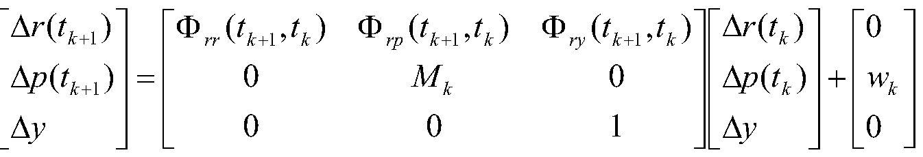 with
with

These matrices are computed for example by integration of the variational equations as described in the section below on numerical orbit integration.
Mk is the matrix describing the stochastic noise modeling
wk is the noise input
Part 8.3 Numerical orbit integration
The satellite motion in orbit can be described by a second order differential equation system x = x(x,x,q) (52)
Appendix A
acceleration in the inertial reference frame
position in the inertial reference frame
velocity in the inertial reference frame
vector of satellite dependent force model unknowns and initial position/velocity
The vector <$ is defined as
 where
where
r(t0 ) are the initial position and velocity in inertial reference frame
a is the vector with dynamic force model parameters
Satellite position x(t) and velocity x(t) at time t are derived from satellite position x(t0 ) and velocity x(t0 ) at time t0 using, for example, a numerical integration (a predictor-corrector method of higher order).
x(t) = x(t0 ) + j"x( <* (54) x{t) = x(t0 ) + ji( <* (55)
The real-time filter uses the partial derivatives of the accelerations x(t) with respect to the unknown parameters q
(56)

The equation of this example ignores derivatives with respect to satellite velocity since there are no relevant velocity -dependent forces acting on GNSS satellites in medium earth orbit.
Appendix A
The following matrix is computed for epoch ti : dx
<ί\<Χ· ) (57) dx
The matrix for the next epoch tM can then be computed via the chain rule Φ ,? ( Wo ) = Φ ,? )Φ ,? ( o ) (58)
The partial derivatives of the observations with respect to the unknowns q can again be derived via chain rule dl dl
— =— Φ, (59) dq dr rq
These partials are used in the observation update of the filter.
The following models are used to compute the accelerations x acting on the satellite; some embodiments use these for the integration process:
1. The Earth's gravity field is modeled by available models such as the EIGEN-CGOIC or the EGM96 model. These are spherical harmonic expansions with very high resolution. Some embodiments use up to degree and order 12 for orbit integration.
2. Gravitational forces due to the attraction by sun, moon and planets.
3. The gravitational forces of sun and moon acting on the Earth's figure will deform the
Earth. This effect also changes the gravity field; it is called "Solid Earth Tide" effect. Some embodiments follow the recommendations of the IERS Conventions 2003.
4. Some embodiments account for the Solid Earth Pole Tide, caused by the centrifugal effect of polar motion. This tide must not be confused with Solid Earth Tides. Some embodiments follow the recommendations of the IERS Conventions 2003.
Appendix A
5. The gravitational forces of sun and moon acting on the oceans will change the gravity field; this is called the "Ocean Tide" effect. Some embodiments use the CSR3.0 model recommended by the IERS Conventions 2003.
6. Some embodiments also consider the relativistic acceleration, which depends upon
position and velocity of the satellite.
7. The solar radiation pressure, the acceleration acting on GNSS satellites, is most difficult to model. Some embodiments consider three components: a first component in the sun- satellite direction, a second component in the direction of the solar radiation panel axis (y-bias) and a third component perpendicular to the first two axes.
8. Some embodiments also model residual errors mainly induced by the insufficient
knowledge of the force models via harmonic functions as described in the following.
GNSS satellites like GPS, GLONASS, GALILEO and COMPASS satellites are in mid earth orbits (MEO) of approximately 26000 km. The following table shows the accelerations acting on GNSS satellites and their effects after a one-day orbit integration.
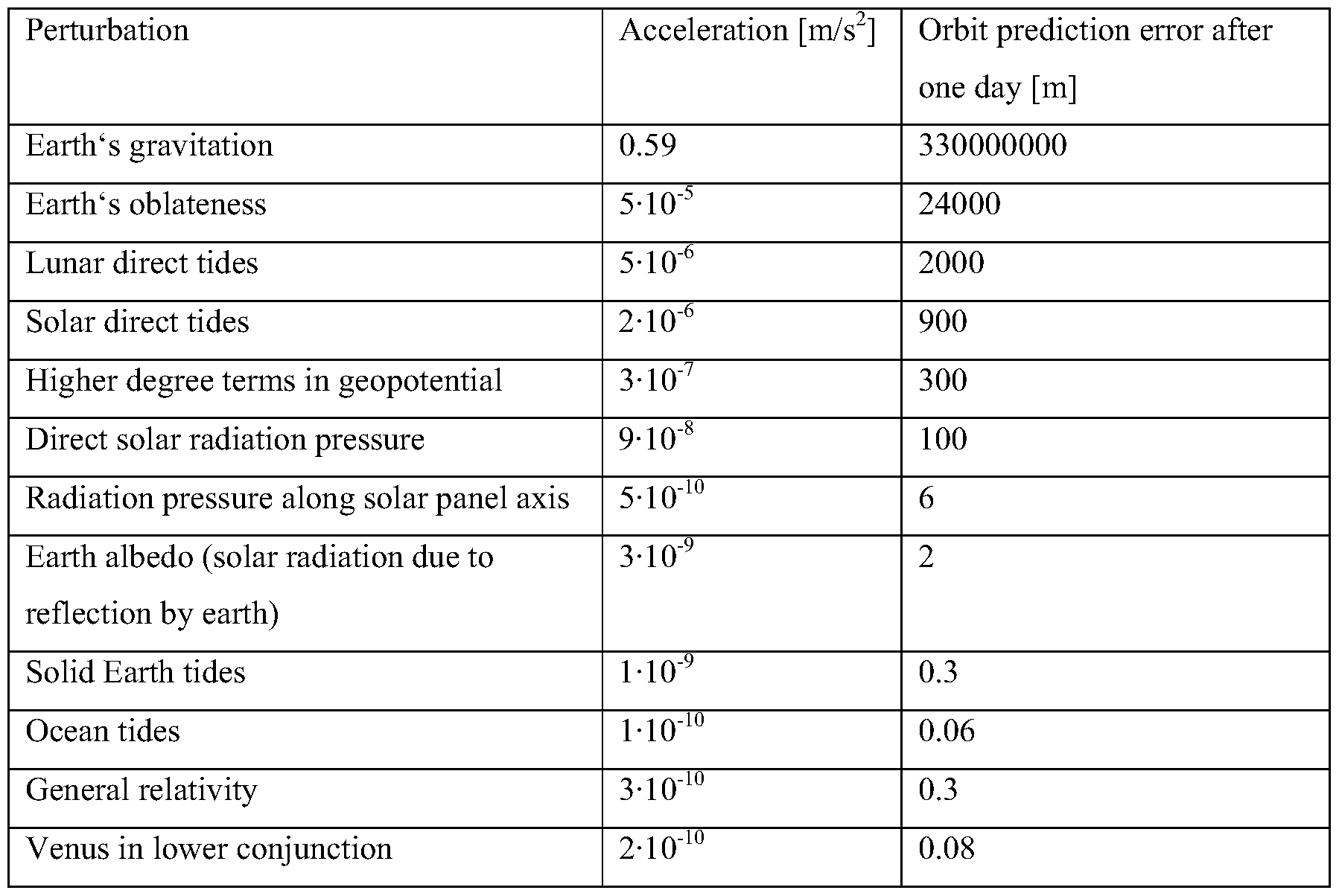
Part 8.4 Harmonic Force Modeling
Some embodiments handle residual errors by introducing a harmonic model having a cosine term and a sine term in each of the along -track, radial and cross-track directions. As the residuals have a period of about one revolution of the satellite about the Earth, the harmonics depend on the argument of latitude of the satellite:

A5 cos + A6 ) with
ΑΆ .. amplitudes to be estimated for along-track
A>A .. amplitudes to be estimated for cross-track
A>A .. amplitudes to be estimated for radial component
... argument of latitude of the satellite
Alternatively to the use of along track, cross track and radial components, the satellite related system (sun-satellite direction, solar panel direction and the normal to both) can be used, to model solar radiation pressure.
Part 8.5 Transformation from Inertial to Earth-Fixed Reference Frame
Some embodiments transform from Inertial to the Earth- fixed reference frame using the IAU 2000A precession/nutation formulas, which follow the IERS Conventions 2003.
Part 8.6 Earth orientation parameters
Some embodiments take Earth orientation parameters (EOPs) from the IERS rapid files
GPSRAPID.DAILY. These files are provided by IERS on a daily basis and are based on the combination of the most recently available observed and modeled data (including VLBI 24-hour and intensive, GPS, and AAM (Atmospheric Angular Momentum)). The combination process
Appendix A
involves applying systematic corrections and slightly smoothing to remove the high frequency noise. GPSRAPID.DAILY contains the values for the last 90 days from Bulletin A for x/y pole, UT1-UTC, dPsi, dEps, and their errors and predictions for next 15 days at daily intervals. After the interpolation, UT1 is corrected for diurnal and/or semidiurnal variations due to Ocean Tides. The polar motion angles are corrected for diurnal variations due to tidal gravitation for a non-rigid Earth, as well as for diurnal and/or semidiurnal variations due to Ocean Tides.
Corrections are computed according to: AA = JB4f s 0/ + C4f∞s 0/ , A {UT\,xP ,yP } (61)
Amplitudes BAf CAf for 41 diurnal and 30 semi-diurnal Ocean Tidal constituents are listed in tables 8.2 and 8.3 in the IERS Conventions (2003). The EOPs from the GPSRAPID.DAILY are introduced as approximate values for the real-time estimation process, keeping linearization errors at a minimum.
Part 8.7 Startup of the Real-Time System
When starting the system for the first time or after interruptions of more than a day, some embodiments derive initial values for satellite position velocity and force model parameters using satellite broadcast ephemerides or IGU orbits. Some embodiments use a least-squares fit to adapt a numerically integrated orbit to the broadcast elements from the satellite navigation message or to the IGU orbit for the satellite. The adapted orbit initial state is then integrated for a time period of up to two days into the future. The satellite positions, velocities and partials are stored in a "partials" file for use by the real-time system.
FIG. 26A shows an embodiment of the startup process 2600 for the real-time orbit processor. An orbit integrator 2605 predicts the orbital states (position and velocity) of each satellite into the future starting from an approximate orbit vector 2615, an initial state taken for example from the broadcast satellite ephemeris or the IGS ultra-rapid orbit IGU by using numerical integration and modeling all relevant forces acting on the satellites, e.g., predicted Earth orientation parameters from IERS. During this process an orbit prediction 2620 is generated, which holds all predicted
Appendix A
orbital states and the partial derivatives. In a next step an adaptation process fits the predicted orbit to the broadcast orbit or IGU orbit via a least squares batch process. This process is iterated until the initial orbital states for the satellites are no longer changing. Then the partials file 2620 is forwarded to the real-time real-time orbit process 2630 of FIG. 26B.
FIG. 26B shows an embodiment of a real-time orbit process 2630. Process 2630 obtains values for an initial start vector 2635 from partials file 2635; these values are used to construct predicted observations for an iterative filter 2640 on a regular basis, e.g., every 150 seconds. Iterative filter 2640 is, for example, a classical Kalman filter or a UD factorized filter or a Square Root Information Filter (SRIF} The orbit start vector 2635 contains the partial derivatives of the current orbit state and force model parameters with respect to the start vector and EOPs and are used to map the partials of the observations to the start vector and force model unknowns.
Kalman filter 2640 receives iono-free linear combinations 2645 of observation data from the reference stations in real time, e.g., each epoch, such as once per second, and predicted Earth orientation parameters (EOP) 2610. With each observation update, Kalman filter 2640 provides improved values for the state vector parameters: receiver clocks 2655 (one per station), zenith tropospheric delays 2660 (one per station), satellite clocks 2665 (one per satellite), optional satellite clock rates 2670 (one per satellite), and orbit start vectors 2680 (one orbit start vector per satellite). In the embodiment of FIG. 26B, orbit state vector 2680 is supplied from time to time (e.g., each epoch, such as once per second) and mapped via the orbit mapper 2682 to the current- epoch orbit position/velocity vector 350.
Orbit mapper 2682 uses the partial derivatives from the partials file and the following relationship to derive satellite position and velocity at the current epoch t; from the state vector at epoch t0 .(Fig 26C). r{t, ) = r0 (f , ) + Φ rq (tt , t0 )xqs (t0 ) = r0 (tt ) + (62)

with
... reference trajectory (position and velocity) created by a numerical orbit integrator
Appendix A
. partials of the position and velocity at tt with respect to the start vector
Xas (to ) at tt estimated difference of the start vector (state vector) at t{
Next r tj ) which is given in the inertial reference frame is transformed into the Earth centered / Earth fixed reference frame.
The current-epoch orbit position/velocity vector 350 in the Earth centered / Earth fixed reference frame is forwarded to the standard clock processor 320, to the phase clock processor 335 and to the scheduler 355 of FIG. 3.
Some embodiments of process 2630 avoid linearization errors by restarting the numerical integration in an orbit integrator 2685 from time to time, such as every 6 or 12 or 24 hours. Orbit mapper 2684 uses the partial derivatives from the partials file and the following relationship to derive a new orbit state vector 2690 in the inertial reference frame at time tn + x hours from the start vector at epoch t0 (Fig 26D).

with
r0 {tt ) ... reference trajectory (position and velocity) created by a numerical orbit integrator
Φ ... partials of the position and velocity at ti with respect to the start vector
x (t0 ) ... at ti estimated difference of the start vector (state vector) at t0 Predicted EOPs 2610 (e.g., from IERS) and estimated EOPs together with updated new orbit start vector 2690 are used as inputs to orbit integrator 2685 to transform coordinates between the inertial frame and the earth-fixed frame, e.g., following the IERS Conventions.
Appendix A
This numerical integration runs in the background and generates a new partials file 2635 which is used to update the predicted observations of Kalman filter 2640. The start vector for the numerical integration of orbit integrator 2675 is for example the latest best estimate of the realtime system, orbit start vector 2690.
Part 8.8 Fixing ambiguities in Real-Time Orbit Determination
Kalman filter 2640 uses the ionospheric-free dual-frequency combinations 2645 of the LI and the L2 GNSS observations. The ionospheric-free combination usually leads to a very small wavelength

(64) The factors i^ and F2 are given in Table 3. For example, for GPS LI and L2 frequencies with Fl = 77 , F2 = 60 and 1 = 0.1903w7 the resulting iono-free wavelength is
F
λ1Ρ = λγ— -— -— - « 6mm . This is below the noise level of the phase observations so that there is no possibility to directly fix the iono-free ambiguity to the correct integer value. Notice that for the iono-free combination between L2 and L5 the iono-free wavelength is with X1F « 12.47cm large enough for reliable ambiguity resolution.
To make use of the integer nature of the LI and L2 ambiguities one could try to solve for the LI and L2 ambiguities, which is difficult due to the unknown ionospheric contribution to the LI and L2 carrier phase observations at the stations. A preferred approach is to solve for carrier-phase ambiguities by fixing the widelane ambiguities NWL := Nl—N2 in a first step. . Substituting N2 in (64) by N2 = Nl - NWL results in
Appendix A
with :■

using the float value from the filter for λΙΡΝΙΡ . After fixing the Nx ambiguity vector to integer or hted average of integer values it can be reinserted into (65) to get a fixed value for
In some embodiments the widelane ambiguities NWL are computed in the widelane bias processor 325 and are transferred to the orbit processor 2630 for example every epoch. For embodiments in which the orbit processor 2630 processes ionospheric-free observations, the ambiguities estimated are ionospheric-free ambiguities λΙΡΝΙΡ .
For embodiments in which the widelane ambiguities NWL are provided by the MW bias processor 325, equation (65) can also be used to reformulate the Kalman filter equations (by subtracting [AWL - ANL )NWL from the observations) and estimate the NT ambiguities directly.
As an alternative to resolving the NT ambiguity with a given integer widelane ambiguity, the equations above can be formulated such that N2 or narrowlane ambiguities are estimated instead; the approaches are equivalent because all these ambiguities are linearly related.
Some embodiments of ambiguity "fixing" mechanism 2695 employ any suitable techniques known in the art, such as Simple rounding, , Bootstrapping , Integer Least Squares based on the Lambda Method, or Best Integer Equivariant (Verhagen, 2005, Teunissen and Verhagen, 2007) The term "fixing" as used here is intended to include not only fixing of ambiguities to integer values using techniques such as rounding, bootstrapping and Lambda search, but also to include forming a weighted average of integer candidates to preserve the integer nature of the ambiguities if not fixing them to integer values. The weighted average approach is described in detail in unpublished patent applications PCT US2009/004476, PCT US2009/004472,
Appendix A
PCT/US2009/004474, PCT/US2009/004473, and PCT/US2009/004471 which are incorporated herein by this reference.
Analyses have shown that the orbit quality is significantly improved by "fixing" the ambiguities, either as integer values or as weighted averages of integer candidates.
Part 8.9 Orbit Processing at IGS Analysis Centers
GNSS orbit determination is done by a variety of IGS Analysis Centers. To our knowledge none of these Centers provides real-time orbit estimation as proposed here.
The CODE Analysis Center (AC) uses a batch least squares approach as described in Dach et al. (2007) and not a sequential filter implementation as described here. Details on the modeling are also described in Beutler et al. (1994). The CODE AC participates in the generation of the IGS Ultra-rapid orbits (IGU). Orbit positions correspond to the estimates for the last 24 hours of a 3- day long-arc analysis plus predictions for the following 24 hours. This is done every 6 hours while the processing and prediction time span is shifted by 6 hours in each step.
The Geoforschungszentrum GFZ estimates orbits and computes a contribution to the IGS Ultra- rapid orbits. The approach is documented by Ge et al. (2005, 2006). Their processing and that of the CODE process is based on a batch least squares approach. GFZ does ambiguity resolution, but only in post-processing mode. No attempt is documented on real-time efforts involving a sequential filter. The European Space Operation Centre ESOC of ESA also contributes to the IGS Ultra-rapid orbit computation. The approach is documented by Romero et al. (2001) and Dow et al. (1999). The approach is also based only on a prediction of satellite orbits. No true real-time processing is done. The Jet Propulsion Laboratory JPL, USA, determines GPS satellite orbits with their system based on the GIPSY-OASIS II software package developed for the US Global Positioning System, general satellite tracking, orbit determination and trajectory studies. Details are published in US Patent 5,963,167 of Lichten et al. The JPL system allows a fully automatic operation and
Appendix A
delivery of validated daily solutions for orbits, clocks, station locations and other information with no human intervention. This data contributes to the orbits published by the IGS including the Ultra-rapid orbit service providing IGU orbits. US Patent 5,828,336 of Yunck et al. describes the implementation of a real-time sequential filter.
The approach of embodiments of the present invention differs from that of US Patent 5,828,336 in at least these ways:
the approach described in US Patent 5,828,336 appears to use smoothed pseudo-ranges only; an example observation update rate given is 5 minutes
- the JPL system described in US Patent 5,828,336 does not appear to fix carrier-phase ambiguities
the approach of US Patent 5,828,336 uses an ionospheric model Part 8.10 References
Beutler, G., E. Brockmann, W. Gurtner, U. Hugentobler, L. Mervart, and M. Rothacher (1994), Extended Orbit Modeling Techniques at the CODE Processing Center of the International GPS Service for Geodynamics (IGS) .'Theory and Initial Results, Manuscripta Geodaetica, 19, 367-386, April 1994.
Bierman, Gerald J. (1977): Factorization Methods for Discrete Sequential Estimation, Academic Press, Inc., New York
Dach, R., U. Hugentobler, P. Fridez, M. Meindl (eds.) (2007), Documentation of the Bernese GPS Software Version 5.0, January 2007
Dow, J., Martin-Mur, T.J., ESA/ESOC Processing Strategy Summary, IGS Central Bureau web site, igscb.jpl.nasa.gov/igscb/center/analysis/esa.acn, 1999 Ge, M., G. Gendt, G.Dick and F.P. Zhang (2005), Improving carrier-phase ambiguity resolution in global GPS, Journal of Geodesy, Volume 80, Number 4, July 2006, DOI: 10.1007/s00190-005- 0447-0
Appendix A
Ge, M., G. Gendt, G.Dick, F.P. Zhang and M. Rothacher (2006), A new data processing strategy or huge GNSS global networks, Journal of Geodesy, Volume 79, number 1-3, June 2005, DOI: 10.1007/sOO 190-006-0044-x Landau, Herbert (1988): Zur Nutzung des Global Positioning Systems in Geoddsie und
Geodynamik: Modellbildung, Software-Entwicklung und Analyse, Heft 36 der Schriftenreihe des Studiengangs Vermessungswesen der Universitat der Bundeswehr Miinchen, Dezember 1988
Lichten, S., Yoaz Bar-Sever, Winy Bertiger, Michael Heflin, Kenneth Hurst, Ronald J.
Muellerschoen, Sien-Chong Wu, Thomas Yunck, James Zumberge (1995) GIPSY-OASIS II: A HIGH PRECISION GPS DATA PROCESSING SYSTEM AND GENERAL SATELLITE ORBIT ANALYSIS TOOL, Proceedings of NASA Technology Transfer Conference, Oct 24-26, 1995, Chicago, 111. Lichten, Stephen M., Wu Sien-Chong, Hurst Kenneth, Blewitt Geoff, Yunck Thomas, Bar-Sever Yoaz, Zumberge James, Bertiger William I., Muellerschoen Ronald J., Thornton Catherine, Heflin Michael (1999), Analyzing system for global positioning system and general satellite tracking, United States Patent 5963167, October 5, 1999. McCarthy, Dennis D. and Gerard Petit (2003), IERS CONVENTIONS, IERS (International Earth Rotation Service) Technical Note 32, October 2003
Romero, I., C. Garcia Martinez, J.M. Dow, R. Zandbergen (2001), Moving GPS Precise Orbit Determination Towards Real-Time, Proceedings GNSS 2001, Seville, Spain, May 2001.
Yunck, Thomas P., William I. Bertiger, Stephen M. Lichten, Anthony J. Mannucci, Ronald J. Muellerschoen, Sien-Chong Wu, (1998), Robust real-time wide-area differential GPS navigation, US Patent 5828336, October 27, 1998.
Teunissen, PJ.G, S. Verhagen (2009); GNSS Carrier Phase Ambiguity Resolution: Challenges and Open Problems, In M.G. Sideris (ed.); Observing our Changing Earth, Inteernational Association of Geodesy Symposia 133, Spinger Verlag Berlin-Heidelberg 2009.
Appendix A
Verhagen, Sandra (2995): The GNSS integer ambiguities: estimation and validation, Publications on Geodesy 58, Delft, 2005. 194 pages., ISBN-13: 978 90 6132 290 0. ISBN-10: 90 6132 290 1.
Appendix A
Part 9: Phase Clock Processor
Referring to FIG. 3, the phase clock processor 335 receives as input MW biases ¾^ 345 (one per satellite) and/or widelane ambiguities Ni J WL 340 (one per satellite-receiver pair), precise orbit information 350 (one current orbit position/velocity per satellite), troposphere information 370 (one troposphere zenith delay per station), low-rate code leveled clocks 365 (one low-rate code- leveled clock error per satellite) and the reference-station GNSS observation data 305 or 315. The phase clock processor 335 generates from these inputs the computed high-rate code-leveled clocks 375 (one high-rate code-leveled clock error per satellite) and the high-rate phase-leveled clocks 370 (one high-rate phase-leveled clock error per satellite), and forwards the MW biases 345 (one per satellite).
Part 9.1 Determining WL Ambiguities from MW Biases Neglecting multipath, a useful characteristic of the Melbourne- Wiibbena (MW) linear combination <$) WL— Pi 1 m is that, aside from some remaining noise i J MW , only the satellite MW biases Wuw and the receiver MW biases bi MW and the widelane ambiguity term hWLNi WL remain: p 4- s-i
^ i,WL 1 i,NL ui,MW υ UW ^ '^WL l i,WL i,MW (66) To get rid of the noise (MW , the Melbourne-Wiibbena linear combination for each satellite is in some embodiments reduced by the satellite MW bias bM J W for that satellite and smoothed (e.g., averaged) over time. Single-differencing between satellites then cancels out the receiver MW bias bi , leaving only a single-differenced widelane ambiguity term per satellite-receiver- satellite connection. The single-differenced widelane ambiguities are computed using the (constant) widelane wavelength XWL . Since only single-differenced widelane ambiguities are used in the phase clock processor, this method is in some embodiments used as a substitute for using the widelane ambiguities 340 from the MW bias processor 325 and/or for a quality check on the widelane ambiguities 340 received from the MW bias processor 325.
Appendix A
Part 9.2 Single-Differenced Phase-Leveled Clocks
The location of each reference station is precisely known. The precise location of each satellite at each epoch is given by the current orbit position/velocity data 350 from orbit processor 330. The geometric range pf between a satellite j and a reference station i at each epoch is calculated from their known locations. The tropospheric delay 77 for each reference station is received from the code clock processor 320.
The ionospheric-free linear combination
(67)
® ijF = Pi + - cAti + T + AjpN-jp + ε, IF is reduced by the (known) geometric range pf and the (known) troposphere delay T , leaving as unknowns only the ionospheric-free ambiguity term lIFNi J IF - λΝΙΝ}χ + -^{λπι - λΝΙ ), the satellite phase clock error term cAtJ := cAt + bJ IF and the receiver phase clock error term οΑίφ . := cAt + b^i IP .
Single-differencing the observations of two satellites at the same receiver cancels out the receiver clock error. Reducing this single difference by the according single difference widelane ambiguity leads to the single difference phase clock together with a single difference Nt ambiguity (often also called narrowlane ambiguity in this context since its corresponding wavelength here is 1NL ).
(68)
 This is computed for each station observing the same pair of satellites. At this point it is
;™ „„; i„ <-„ Λ :„\, i „: 1„ A: CC „„<-„n;<-— 1— 1,„™ i „: 1„
Appendix A
difference narrowlane ambiguity term, which is an integer multiple of the narrowlane wavelength. If the single difference ambiguity is set to zero a single difference phase clock
 shifted by an integer number of narrowlane cycles is achieved. This phase clock has a non fixed narrowlane status. The difference of two of those single difference clocks is an integer number of narrowlane cycles.
Part 9.3 Smoothed Single-Differenced Phase Clocks
For each pair of satellites, the single-differenced phase clock errors observed from different stations shifted to a common level using fixed narrowlane ambiguities is averaged to get a more precise clock error:

Part 9.4 Phase Clock Estimation
Part 9.4.1 Spanning-Tree-Based Phase Clocks
Some embodiments use a spanning-tree approach to estimate phase-leveled clocks. To compute a single-differenced clock error between any arbitrary pair of satellites, a set of single difference- phase clocks is needed for the satellite-to-satellite links such that there is a unique path to reach each satellite via satellite-to-satellite links starting from a dedicated reference satellite. If all satellites are nodes of a graph, such a path is called spanning tree. If each edge of the graph is equipped with a weight, a minimum spanning tree is a spanning tree with a minimal sum of edge weights. Some embodiments use a discrete category based weighting scheme for an edge between two satellites and assign the following phase clock values to the edge:
i Several edges connecting satellites
 and j2 have a fixed Nl ambiguity:
Appendix A
and j2 have a fixed Nl ambiguity:
Appendix A
ii Only a single edge connecting satellites and j2 has a fixed Nl ambiguity: cA7Jj2 + λ Nh
iii No edge connecting satellites
 and j2 has a fixed Nl ambiguity : cAtJ1 1 for receiver / with min(elevation(j l,j2) is maximal.,
iv No WL ambiguity available for edge connecting satellites
 and j2 : Don't use such an edge; thus no phase clock has to be defined;
Each edge of category (i) has a lower weight than an edge of category (ii), each edge of category (ii) has a lower weight than an edge of category (iii) etc. Edges within each category have a continuous weight that is in some embodiments derived in category (i) from the variance of the average and in category (ii) and (iii) from the elevations under which the satellites in the single difference are seen at the corresponding station.
If the minimum spanning tree uses an edge without a fixed narrowlane status, the narrowlane ambiguity N^ 1 is set to zero and achieves fixed status. Choosing a reference satellite with phase clock error cAt^ set to zero, single-differenced phase clock errors cAtJref[Jl to all other satellites are computed solving a linear system. The satellite's phase clock error is then defined as cAt^ := cAt^ Part 9.4.2 Filter Estimation of Phase Clocks
Some embodiments use a filter approach to estimate phase-leveled clocks. A filter is set up with all satellite phase clock errors as states. The state of the reference satellite's clock error cAt^ef is set to zero. In some embodiments all links from the spanning tree and in addition all links with fixed narrowlanes are added to the filter to estimate more precise single-differenced phase clock errors.
Part 9.5 Narrowlane Filter Bank
Appendix A
Once a set of single-differenced phase clock errors is estimated, e.g., as in Part 9.4, all observations for shifted single-differenced phase clocks in Part 9.2 are reduced by the clock errors estimated in Part 9.4:

What remains is an observable for the integer narrowlane offset. For each station a narrowlane filter with a narrowlane ambiguity state per satellite is updated with those observations.
Part 9.6 High-Rate Single-Differenced Code-Leveled Clocks
The phase clock processor 335 also computes high-rate code-leveled clocks.
Part 9.6.1 Buffering Low-Rate Code-Leveled Clocks GNSS observations (reference station data 305 or 315) for a time (e.g., an epoch) tl are buffered for use when the low-rate information with the same time tag ( tl ) arrives from the code-leveled clock processor 360; this information comprises two of: clock errors 365, tropospheric delays 370, and ionospheric-free float ambiguities 374. Thus, GNSS observations matched in time with the low-rate clock processor information are always available from an observation buffer. When a set of low-rate code leveled clocks 365 arrive they are combined with the GNSS observations and with the tropospheric delays 370 and with time-matched satellite position/velocity information 350 to compute the carrier ambiguities.
FIG. 27A shows at 2700 the flow of data for the case where the satellite clocks (clock errors) 365 and the tropospheric delays 370 are used. GNSS observations arrive over time at the phase clock processor 335 with (e.g. epoch) time tags t0 , tl , t2 , t3 , etc. Low-rate code leveled clocks cAtp J and tropospheric delays T arrive asynchronously over time with time tags t0 , tl , t2 , t3 , etc. An observation buffer 2705 holds the observations. These are combined for each time ti in a combiner 2710 with satellite position/velocity data, with the low-rate code-leveled clocks c tj,
Appendix A Nf := hIFNfIF + 6Φ)!-)ΙΡ - bP i.IF - - bP IF ). A process 2715 computes the single- differenced code-leveled clocks 2720.
FIG. 27B shows at 2715 the flow of data for the case where the ionospheric-free float ambiguities 374 and the tropospheric delays 370 are used. GNSS observations arrive over time at the phase clock processor 335 with (e.g. epoch) time tags t0 , tl , t2 , t3 , etc. Ionospheric-free float ambiguity terms INf and tropospheric delays T arrive asynchronously over time with time tags to , tl , t2 , t3 , etc. An observation buffer 2720 holds the observations. These are combined for each time ti in a combiner 2710 with the ionospheric-free ambiguity terms N- , with the low- rate code-leveled clocks c tp J and with the tropospheric delays T to produce the ionospheric-free a ambiguity terms INf . A process 2740 computes the single-differenced code-leveled clocks 2720.
Part 9.6.2 Computing Ambiguities in the Phase Clock Processor
The data combiner (2710 or 2735) forms an ionospheric-free linear combination of the carrier- phase observation, and reduces this by the geometric range pf (computed using the receiver and satellite positions), the tropospheric delay T and the low-rate code-leveled satellite clock error c tj, (e.g., clocks 365). After this reduction the receiver clock error and a float ambiguity remains. If this is done using between-satellite single-differenced observations, the receiver clock is eliminated and thus only the single-differenced ionospheric-free ambiguity term remains:
Φ (Ί) - Pt'h (Ί) - 'h (Ί) + c t^ ft) = AN^ ( + ^( _ (72) with cAtp Jlh := cAthh + bp J and float ambiguity XNjih := λσ Ν^ - - bp J ) which is a constant value and is kept to be used until the next update of low rate clocks.
As an alternative to computing the ionospheric-free ambiguities in the phase clock processor 335, the ionospheric-free float ambiguities are obtained from a previous processor, such as
Appendix A
Part 9.6.3 Using Iono-Free Ambiguities to Compute High Rate Code Clocks
Once iono-free ambiguities are known for time il , single-differenced ionospheric-free linear combinations at any time in the future ( e.g. t2 ) can be used for each pair of satellites along with tropospheric delay and current geometric range:
(73)
Φ ('2) - p 'h (k) - T Jl (k) - h ( = -c ^ (k) + ^IM + *#>(
The result of this computation is the single-differenced phase-leveled satellite clock error cttp 31 . With this it is possible to estimate high-rate single-differenced code-leveled clock errors cAtp refJl between a given satellite j2 and a chosen reference satellite jref . If only the between-satellite single-differenced clock errors are of interest, the reference satellite clock error c tp Jrer is set to zero.
FIG. 28A shows a first embodiment 2800 for preparing the undifferenced (also called ZD or Zero-Differenced) high-rate code-leveled satellite clocks 375. Precise satellite orbit information, e.g., satellite position/velocity data 350 or 360, and GNSS observations, e.g., reference station data 305 or 315, are supplied as inputs to a first process 2805 and as inputs to a second process 2810. The first process 2805 estimates a set of ionospheric-free float ambiguities 2815. These are supplied to the second process 2810 which estimates the undifferenced high-rate code-leveled satellite clocks (clock errors) 375.
FIG. 28B shows a second embodiment 2820 for preparing the undifferenced (also called ZD or Zero-Differenced) high-rate code-leveled satellite clocks 375. Precise satellite orbit information, e.g., satellite position/velocity data 350 or 360, and GNSS observations, e.g., reference station data 305 or 315, are supplied as inputs to a low-rate code-leveled clock processor 2825, e.g., code clock processor 320, and as inputs to a high-rate code-leveled clock processor 2830. The low- rate code-leveled clock processor 2825 prepares ionospheric-free float ambiguities 2835, e.g., ionospheric-free float ambiguities 374, and tropospheric delays 2840, e.g., tropospheric delays 370. The ionospheric-free float ambiguities 2835 and the tropospheric delays 2840 are supplied
Appendix A
to the high-rate code-leveled clock processor 2830, e.g., forming a part of phase clock processor 335. The high-rate code-leveled clock processor 2830 uses the inputs at 2845 to compute single- differenced high-rate code-leveled satellite clocks 2850. A filter 2855 uses these to estimate undifferenced high-rate code-leveled satellite clocks (clock errors) 2860, e.g., high-rate code- leveled satellite clocks 375.
FIG. 28C shows a third embodiment 2865 for preparing the undifferenced high-rate code-leveled satellite clocks 375. Precise satellite orbit information, e.g., satellite position/velocity data 350 or 360, and GNSS observations, e.g., reference station data 305 or 315, are supplied as inputs to a low-rate code-leveled clock processor 2870, e.g., code clock processor 320, and as inputs to a high-rate code-leveled clock processor 2875. The low-rate code-leveled clock processor 2870 prepares low-rate code-leveled clocks 2880, e.g., low-rate code-leveled satellite clocks 365, and tropospheric delays 2882, e.g., tropospheric delays 370. The low-rate code-leveled satellite clocks 2880 and the tropospheric delays 2882 are supplied to the high-rate code-leveled clock processor 2875, e.g., forming a part of phase clock processor 335. The high-rate code-leveled clock processor 2884 uses the inputs at 2884 to compute ionospheric-free float ambiguities 2886 which are used at 2888 to compute single-differenced high-rate code-leveled satellite clocks 2890. A filter 2892 uses these to estimate undifferenced high-rate code-leveled satellite clocks (clock errors) 2894, e.g., high-rate code-leveled satellite clocks 375.
Part 9.6.4 Clock Shifter
Single-differenced phase-leveled clock errors cAt^Jl and single-differenced code-leveled clock errors c tp refJl are estimated as in the course of estimating phase-leveled satellite clocks and high-rate single-differenced code-leveled satellite clocks. The single-differenced high-rate code- leveled satellite clocks have the same accuracy as single differences of the low-rate code-leveled satellite clocks. The phase-leveled satellite clocks are constructed to preserve the integer nature of the narrowlane ambiguity if used for single-differenced ionospheric-free carrier-phase observations together with the precise satellite orbits and the widelane ambiguities, derived from the MW biases, used in the clock estimation. Thus the quality of a single-differenced phase- leveled clock error is not changed if this clock error is shifted by an integer number of narrowlane cycles. Since the phase-leveled satellite clock errors will always be used in a single difference, such a shift which is applied all satellite clock errors will cancel out again in the single-
Appendix A
differencing operation. In accordance with some embodiments the following shift is applied to the phase-leveled satellite clock errors to keep their values close to the low-rate code-leveled satellite clock errors and reduce their noise.
Thus in some embodiments an integer number of narrowlane cycles
In some embodiments the low-rate code-leveled clock errors are approximated with a continuous steered clock cAt P , steered . The value of the steered clock of the reference satellite
= c A i P , steered (75) is then added to all high-rate clocks. Doing so, all clocks are close to the code-leveled low-rate clocks, but the reference clock is smooth.
In some embodiments the mean of the difference between the high-rate phase-leveled satellite clocks and their corresponding steered low-rate clock is computed and added to all shifted phase- leveled satellite clock errors. The same is done for the high-rate code-leveled satellite clocks. This procedure pushes some noise into the reference clock.
P .noise
Φ .noise

r\t Φh = r <-ί\Λtιφmf + ^ Α v , noise + ^ A v ref + ^ A tNrL4
The shifting is mainly done to keep the phase-leveled satellite clock errors near GPS time and therefore make certain transmission methods applicable. In addition the clock bias
Appendix A
b{t = cAtP J - cAti (78) which is the difference between the phase-leveled satellite clocks and code-leveled satellite clocks, can be kept within a certain range.
Part 9.6.5 Jump messages
If the clock bias leaves its range or if the phase-leveled clocks' satellite-to-satellite links have been estimated without using fixed narrowlane ambiguities, the shift will change and a jump message is sent. This also means that the phase-leveled satellite clock error changes its level. Part 9.7 Phase Clock Processor Embodiments
FIG. 29 shows an architecture 2900 of a phase clock processor 335 in accordance with some embodiments of the invention. The inputs to the phase clock processor are: MW biases and/or fixed WL ambiguities 2095 (e.g., MW biases 345 and/or fixed WL ambiguities 340), low-rate (LR) code-leveled clocks 2910 (one per satellite, e.g., low-rate code-leveled satellite clocks 365), satellite orbit information (e.g., precise satellite orbit position/velocities 350 and/or IGU orbit data 360), tropospheric delays 2920 (one per reference station, e.g., tropospheric delays 370), and GNSS observations 2925 (of multiple satellites at multiple reference stations, e.g, reference station data 305). The choice of MW biases or fixed WL ambiguities gives two options. A first option is to use the low-rate MW biases together with the low-rate orbit information 2915 and the GNSS observations 2925 in an optional fixer bank 2930 to fix the WL ambiguities. These are then provided at a high rate (HR) as single-differenced fixed WL ambiguities 2935 to a computation process 2940. A second option is use the low-rate fixed WL ambiguities directly to supply single-differenced (SD) fixed WL ambiguities to the process 2940. By high-rate is meant that the single-differenced fixed WL ambiguities used in the high-rate process 2940 remain the same from epoch to epoch in process 2940 between low-rate updates.
The low-rate code-leveled clocks 2910 are used in process 2945 to compute low-rate single- differenced ionospheric-free float ambiguities 2950. These are used with the low-rate orbit data 2915 and the low-rate tropospheric delays 2920 and the high-rate GNSS observations 2925 in a process 2955 to compute single-differenced high-rate code-leveled clocks 2960 (one per satellite,
Appendix A
The high-rate single-differenced fixed WL ambiguities 2935 are used with the low-rate orbit data 2915 and the low-rate tropospheric delays 2920 and the GNSS observations 2925 in a process 2940 which computes high-rate phase-leveled clocks 2945 (one per satellite, such as high-rate phase-leveled satellite clocks 375). The high-rate phase-leveled clocks 2945 are used together with the orbit data 2915 and the tropospheric delays 2920 and the GNSS observations 2925 in an ambiguity fixer bank 2975 which attempts to fix single-differenced ambiguities, e.g., LI ambiguities. The single-diffierenced fixed ambiguities 2980 are pushed into the process 2965 to aid the computation of high-rate phase-leveled clocks 2970.
The MW biases and/or fixed WL ambiguities 2905 and the low-rate code-leveled clocks 2910 and the single-differenced high-rate code-leveled clocks 2960 and high-rate phase-leveled clocks 2970 are fed into a process 2985 which shifts and combines these to deliver a high rate data flow 2990 containing (at least) high-rate phase-leveled satellite clocks, high-rate code-leveled clocks and high-rate MW biases. Data 2990 is supplied to scheduler 355 as described in FIG. 3.
FIG. 30A shows an embodiment 3000 of a process for estimating high-rate phase-leveled satellite clocks. Precise satellite orbit information, e.g., satellite position/velocity data 350 or 360, and GNSS observations, e.g., reference station data 305 or 315, are supplied at low rate as inputs to a first process 3015 and at high rate as inputs to a second process 3020. The first process 3015 estimates ambiguities 3025, one set of ambiguities per receiver. Each ambiguity corresponds to one of a receiver-satellite link and a satellite-receiver-satellite link. These ambiguities are supplied at low rate to the second process 3020 which estimates the high-rate phase-leveled clocks 3030.
In general a linear combination of carrier phase observations has receiver-dependent parameters pr like receiver position, receiver clock error or receiver biases, satellite-dependent parameters p" like the satellite position, and receiver-satellite-link dependent parameters pr s like the tropospheric or the ionospheric delay. Let .s rk , k e l be linear combinations of code and carrier phase observations with wavelength Xk and ambiguity Nr s k . A code and carrier phase combination as assumed here can be written as
Appendix A

with L < L, L not empty and real factors ak e ¾ .
Note that / : 3i"p — > ¾ is linear in most of the parameters. If a mapping exists to convert between a receiver-satellite link dependent parameter and a receiver dependent parameter, it can be used to reduce the number of unknowns. As an example the troposphere delay can be modeled as a delay at zenith, which is mapped to line of sight. Thus instead of having one parameter per receiver-satellite link, only one parameter per receiver is needed.
Using special linear combinations such as an ionospheric-free combination, parameters can be canceled out. Each additional input of at least one of the parameters contained in pr , ps and pr s simplifies and accelerates the estimation process. In satellite-receiver-satellite single differences the parameters pr cancel out. In the following all can be done in single or zero difference, but this will not be mentioned explicitly in each step. If all parameters pr , ps , pr s and cAt" are known and the noise is neglected, the remaining part y^flfr (bk s + AkNr s k ) is not unique without additional information. Setting the ambiguities for a specific satellite-receiver combination to zero will shift the biases accordingly. If the ambiguities are known, the level of the bias is defined; if the bias is known, the level of ambiguities is defined.
In some linear combinations of code and carrier-phase observations the parameter pr , p" , pr s and cAt " cancel out, as do the receiver biases brk . This allows estimating the biases Vk , brk and the ambiguities Nr s k separated from the other parameter.
Not all satellite biases can be estimated separately from the satellite clock error cA . In this case the sum of the real satellite clock and the biases are estimated together and the result is just referred as the satellite clock error. In this case shifting a bias is equivalent with shifting a clock.
Appendix A
In the following a distinction is made between ambiguities belonging to biases and ambiguities belonging to clock errors. The clock ensemble and also the biases ensemble estimated from GNSS observations are underdetermined. Thus one of the satellite or receiver clock errors or any combination of them can be set to any arbitrary value or function to make the system solvable. In some embodiments one of the clocks is set to zero, or additional measurements or constraints for one of the clock errors or a linear combination of clock errors are added. The examples given here always have a reference clock or bias set to zero, for purposes of illustration, but this is not a requirement and another approach can be used. Process I (3015): In a first step all other input parameters are used to reduce the linear combination of carrier phase observations. Depending on the linear combination used, there are small differences in how to estimate phase-leveled satellite clock errors. One option is to use a single, big filter: In this case, all remaining unknown parameters of pr , p" and pr s , the satellite clock errors, including biases, and all ambiguities of are modeled as states in one filter, e.g. a Kalman filter. As an example the filter used for orbit determination in Part 8.
[ORBIT PROCESSOR], the one used for code-leveled clocks in Part 6._
[CLOCK PROCESSOR] (except the integer nature of ambiguities) or the Melbourne-Wiibbena bias processor in Part 8. [WL PROCESSOR] can be used. Another option is to perform a hierarchical estimation.
In some embodiments using linear combinations of code and carrier-phase observations in which the parameters pr , ps , pr s and cAt" cancel out, the biases and ambiguities of estimated in an auxiliary filter and can be used to simplify the main filter. Another option is to use a bank of filters rather than a single filter or rather than a main filter with auxiliary filter. If all parameter beside the ambiguities are known, in at least one of the code and carrier-phase combinations or Ω^ , k e L the ambiguities can be estimated in a filter bank with one filter for each ambiguity or one filter for each receiver. This is done for single- differenced observations in the phase clock processor to estimate the widelane ambiguities using the Melbourne-Wiibbena linear combination and Melbourne-Wiibbena biases as input.
Appendix A
embodiments the results of the filter banks are used to reduce the carrier-phase combinations in the main filter used to estimate the remaining unknowns.
At least one set of fixed ambiguities is sent from process I (3015) to process II (3020), but all the estimated parameters could be sent in addition.
Process II (3025): In process II the linear combination is reduced by all input parameters from process I or additional sources. If no fixed ambiguities are available for the ambiguities from process I that belong to the clock error, a subset of those ambiguities defined e.g. by a spanning tree is in some embodiments set to any arbitrary integer number and used like fixed ambiguities as discussed above. If this subset changes or is replaced by fixed ambiguities of process I, the resulting satellite phase clock errors may change their level. All remaining unknowns are modeled as states in a filter, e.g. a Kalman filter. As in FIG. 3 OA, some embodiments estimate the ambiguities at a first rate and estimate a phase- leveled clock per satellite at a second rate higher than the first rate. The ambiguities estimated in process I (3005) are constant as long the receiver has no cycle slip. Thus an estimated ambiguity can be used for a long time. Also some of the other states like the troposphere estimated in process I (3005) vary slowly and can be assumed to be constant for a while. If the observations of process II (3020) are reduced by those constant and slowly varying parameters, the filter used to estimate clock errors has only a view unknowns left and is therefore quite fast. In general, processor II can work at a higher update rate than process I.
FIG. 30B is a simplified schematic diagram of an alternate phase clock processor embodiment 3035 with WL ambiguities input as in option 2 of FIG. 29 (compare with process 2965). Satellite orbit data 3005 (e.g., 350 or 360), GNSS observations 3010 (e.g., 305 or 315), tropospheric delays 3040 (e.g., 370) and fixed WL ambiguities 3045 (e.g., 340) are supplied to a filter bank 3050 of process I (3015). Filter bank 3050 estimates single-differenced free narrowlane ambiguities 3055. The SD free NL ambiguities 3055 and the fixed WL ambiguities 3045 are combined in a process 3060 with the satellite orbit data 3005, the GNSS observations 3010, and the tropospheric delays 3040 to compute single-differenced satellite clocks 3062. These are applied to a narrowlane filter bank 3064 to estimate single-differenced- satellite clocks 3066. A
Appendix A
satellite clocks 3070. These are fed back to the filter bank 3050 of process I (3015) to improve the estimation of the single-differenced free narrowlane ambiguities 3055.
FIG. 30C is a simplified schematic diagram of an alternate phase clock processor embodiment 3075 with MW biases input as in option 1 of FIG. 29 (compare with process 2965). Satellite orbit data 3005 (e.g., 350 or 360), GNSS observations 3010 (e.g., 305 or 315), tropospheric delays 3040 (e.g., 370) and fixed WL ambiguities 3045 (e.g., 340) are supplied to a filter bank 3078 of process I (3015). Filter bank 3078 estimates single-differenced free narrowlane ambiguities 3088. A filter bank 3082 uses the MW satellite biases 3045 to estimate WL ambiguities 3084. As in FIG. 30B, the SD free NL ambiguities 3055 and the fixed WL ambiguities 3084 are combined in a process 3060 with the satellite orbit data 3005, the GNSS observations 3010, and the tropospheric delays 3040 to compute single-differenced satellite clocks 3062. These are applied to a narrowlane filter bank 3064 to estimate single-differenced- satellite clocks 3066. A spanning tree process 3068 (e.g. MST) is applied to these to produce a set of single-differenced satellite clocks 3070. These are fed back to the filter bank 3078 of process I (3015) to improve the estimation of the single-differenced free narrowlane ambiguities 3080.
FIG. 31 shows an embodiment 3100 in which estimating a phase-leveled clocks per satellite comprises using at least the satellite orbit information, the ambiguities and the GNSS signal data to estimate a set of phase-leveled clocks per receiver, each phase-leveled clock corresponding to one of a receiver-satellite link and a satellite-receiver-satellite link; and using a plurality of the phase-leveled clocks to estimate one phase-leveled clock per satellite. The satellite orbit information 3105 (e.g, 350 or 360) and the GNSS observations 3110 (e.g., 305 or 315) are used in a first process 3115 to determine the ambiguities 3120. The ambiguities 3120 are used with the satellite orbit information 3105 and the GNS S observations 3110 in a second process 3125 to estimate the set of phase leveled clocks 3130, each phase-leveled clock corresponding to one of a receiver-satellite link and a satellite-receiver-satellite link. These are used in a third process 3135 to estimate satellite clocks 3140, one per satellite. Instead of having a big filter, the problem can be decoupled using a small filter for each satellite- to-satellite link to estimate clock errors per receiver-satellite link or in single difference case per satellite-receiver-satellite link. Afterwards those clock errors per link can be combined either
Appendix A
using only links defined by a spanning tree (e.g., as at 3058) or using a filter with one clock error state per satellite.
In some embodiments, the ambiguities are estimated using at least one previously-estimated phase-leveled clock per satellite. As mentioned above, the known fixed ambiguities define the clock error level, and (vice versa) a known clock error leads to ambiguities fitting this clock error. Thus the feedback of clock error estimates to process I allows to estimate ambiguities without having a dedicated clock error state. Since process II can already produce clock error estimates before having all ambiguities fixed, this feedback is advantageous in such a scenario to fix ambiguities belonging to clock errors. Using clock error estimates from a second phase clock processor as input to process I allows to estimate ambiguities fitting those clocks and finally to estimate satellite clock errors at the same level as the other processor's clock errors.
FIG. 32 shows one such embodiment 3200. The satellite orbit information 3205 (e.g, 350 or 360) and the GNSS observations 3210 (e.g., 305 or 315) are used in a first process 3215 to determine the ambiguities 3220. The ambiguities 3220 are used with the satellite orbit information 3205 and the GNSS observations 3210 in a second process 3225 to estimate the set of phase leveled clocks 3230. These are fed back to the first process 3215 where they are used in estimating the ambiguities 3220. For this embodiment it is advantageous to have a secondary clock processor as a back up which is available to immediately provide clock error estimates without level change in case of a failure of the primary clock processor.
In some embodiments at least one additional phase-leveled clock per satellite estimated from an external source is obtained and used to estimate the ambiguities. FIG. 33 shows one such embodiment 3300. In part 3355, the satellite orbit information 3305 (e.g, 350 or 360) and the GNSS observations 3310 (e.g., 305 or 315) are used in a first process 3315 to determine the ambiguities 3320. The ambiguities 3320 are used with the satellite orbit information 3305 and the GNSS observations 3310 in a second process 3325 to estimate the set of phase leveled clocks 3330. In part 3385, the satellite orbit information 3355 (e.g, 350 or 360) and the GNSS observations 3310 (e.g., 305 or 315) are used with one or more of satellite clocks 3330 in a first process 3365 to estimate the ambiguities 3370. In this embodiment part 3335 is an external source of the satellite clocks 3330 with respect to part 3385. The ambiguities 3370 are used with the satellite orbit information 3355 and the GNSS observations 3360 in a second process 3375 to estimate the set of phase leveled clocks 3380.
Appendix A
In some embodiments, at least one set of ambiguities per receiver is determined for additional receivers, each ambiguity corresponding to one of a receiver-satellite link and a satellite-receiver- satellite link. After determining the ambiguities for the additional receivers, at least the precise orbit information, the ambiguities for the additional receivers and the GNSS signal data are used to estimate the at least one additional phase-leveled clock per satellite.
FIG. 34 shows one such embodiment 3400. In part 3455, the satellite orbit information 3405 (e.g, 350 or 360) and the GNSS observations 3310 (e.g., 305 or 315) are used in a first process 3415 to determine the ambiguities 3420. The ambiguities 3420 are used with the satellite orbit information 3405 and the GNSS observations 3410 in a second process 3425 to estimate the set of phase leveled clocks 3430. In part 3485, the satellite orbit information 3455 (e.g, 350 or 360, but optionally from a different orbit processor associated with a different network of reference stations) and the GNSS observations 3410 (e.g., 305 or 315, but optionally from a different network of reference stations) are used with one or more of satellite clocks 3430 in a first process 3465 to estimate the ambiguities 3470. The ambiguities 3470 are used with the satellite orbit information 3455 and the GNSS observations 3460 in a second process 3475 to estimate the set of phase leveled clocks 3480. The primary and secondary clock processors can also be of different kind. This option can be used to estimate the ambiguities close to the level of clock errors based on a different linear combination (e.g. code clock error or different phase combination). Using those ambiguities in process II will lead to clock errors close to clock errors input in process I.
Appendix A
Part 10: Scheduler & Message Encoder
FIG. 35 is a schematic diagram showing a scheduler 355 and a message encoder 385 in accordance with some embodiments of the invention.
Methods and apparatus for encoding and transmitting satellite information are described Patent Application Publication 2009/0179792 Al and 2009/0179793 Al .
Appendix A
Part 11: Rover Processing with Synthesized Reference Station Data
Rodrigo Leandro
Ulrich Vollath
Xiaoming Chen
Part 11.1 Introduction
Existing RTK rover positioning engines are typically designed to process differenced data; the rover data is differenced with base station data and the filters operate on the differenced data. The GNSS observations are contaminated with a number of errors such as satellite clock error, receiver clock error, troposphere delay error, and ionospheric delay error. The satellite-dependent errors (e.g. satellite clock error) can be eliminated if the difference between the observations of two receivers observing the same satellite is used. If those receivers are located close enough to each other (e.g. a few kilometers under normal conditions) then the atmosphere-related errors can also be eliminated. In case of VRS (Virtual Reference Station) the difference is done not between two stations, but between the rover station and a virtual station, whose data is generated using observations from a network of receivers. From this network it is possible to create knowledge of how errors behave over the region of the network, allowing differential positioning over longer distances.
Prior approaches for Precise Point Positioning (PPP) and PPP with ambiguity resolution
(PPP/RTK) remove modeled errors by applying them as corrections (subtracting the errors) to the rover data. Though this works, using a rover receiver configured to process differenced data requires a change in data preparation in that single-differencing has to be replaced by rover-data- only error correction before the data can be processed.
This implies two different modes of operation inside the rover's positioning engine. In practice this results in separate processors for PPP and RTK. This consumes a lot of software development resource, and occupies more of the rover's CPU memory for the additional modules and data.
Appendix A
Part 11.2 Global Virtual Reference Station Positioning
Some embodiments of the invention are based on a substantially different approach, in which a Synthesized Base Station (SBS) data stream is generated for any position on or near the Earth's surface using precise satellite information (e.g., precise orbits and clocks). This data stream is equivalent to having a real reference station near the rover.
For processing at the rover, a Real-Time Kinematic (RTK) positioning engine is used that is adapted to the different error characteristics of PPP as compared to traditional Virtual Reference Station (VRS) processing. Unlike traditional VRS processing, some embodiments of the invention use a processing approach which does not rely on small ionospheric residuals. And in contrast with traditional VRS processing, some embodiments of the invention optionally process different pseudorange observables. PPP and PPP/RTK functionality are retained, with comparatively low software development and few changes in the rover positioning engine, while retaining the advantage of well-proven RTK engines that had been developed and perfected with many man-years of development time. Examples of such functionality include processing of data collected under canopy and dealing with delays in the reference data/corrections (low-latency positioning).
PPP-RTK studies using the SBS technique have proven the high performance of such a system. A positioning accuracy of 10 cm horizontal (95%) was achieved after about 600 seconds (mean) when processing a test data set. Convergence to the typical long baseline and VRS survey accuracy of 2.54 cm horizontal (95%) was achieved after 900 seconds (mean). This suggests that SBS techniques described here can provide sub-inch horizontal-positioning performance.
Part 11.2 Generating SBS Data
The SBS technique enables the generation of virtual GNSS data (data from a virtual GNSS reference/base station) for any position on or near the Earth's surface using precise satellite information (e.g., orbits, clocks). The core of the processing is done inside a module which responsible for the generation of the virtual data. The aim of such data generation is to make it possible to use GNSS satellite precise information in a GNSS receiver running an RTK Engine
Appendix A
(RTK Engine is described in Part [RTK DESCRIPTION]). Therefore the receiver's antenna position is computed by the RTK engine with differential GNSS data processing (i.e. difference between observations of a reference receiver and a rover receiver) using the SBS data as coming from the (virtual) reference receiver, and the rover receiver. The technique therefore allows that a differential GNSS processor is used to compute positions anywhere without the explicit need of a nearby reference station.
The SBS module uses at least one of the following:
• Phase-leveled clocks: These are the satellite clock offsets computed as described in Part 9._ [PHASE CLOCK DESCRIPTION].
• Code-leveled clocks): These are the satellites clock offsets computed as described in Part 6._ [STANDARD CLOCK DESCRIPTION].
• Melbourne-Wuebenna bias: These are the satellite biases for the Melbourne-Wuebenna phase and code combination computed as described in Part 8. [WL BIAS
DESCRIPTION].
• Jump messages: These messages can indicate whether or not the satellite phase clock had a change of level in the recent past (e.g. 10 minutes). The reasons for a level change are pointed out in Part 9._ [PHASE CLOCK DESCRIPTION]. Whenever a jump (level change) occurs in the satellite phase clock offset, some action has to be taken on the rover. This action might be the reset of the satellite's ambiguity(ies) in the RTK engine;
• Approximate rover position: This is the position for which the virtual base data will be generated. The approximate position of the rover can be used for example so that geometric-dependent components (e.g. satellite position) are the same as for the rover data.
· Time tag: This is the time (epoch) for which the virtual data has to be generated. The virtual data has to be created for certain instants of time (epochs) that depend on the rover observation time tags, so that it can be used in the differential data processing together with the rover data.
Given one or more items of the list above as input the SBS module generates as output a set of GNSS virtual observations. These observations comprise and are not restricted to: LI code, L2 code, LI phase, L2 phase, LI cycle slip information, L2 cycle slip information, exact virtual base position. Once the virtual reference station dataset is available it can be
Appendix A
delivered to the RTK engine for differential processing with the rover's own GNSS observation data and optionally using the precise satellite data. The RTK engine can then apply conventional RTK processing to compute the rover coordinates (see Part [RTK
DESCRIPTION]).
Part 11.3 Moving Base
The best corrections for kinematic rovers are obtained when the SBS position and the synthesized reference station data for the SBS position are updated frequently, e.g., for every epoch of rover observations a new set of SBS data is generated. Some embodiments use as the SBS position a first estimate of the rover position, derived for example from a simple navigation solution using the rover observations.
In the case of prior-art Virtual Reference Station (VRS) processing, a moving rover can result in a significant separation between the rover position and the VRS location for which the VRS data is synthesized. Some implementations mitigate this by changing the VRS position when this distance exceeds a certain threshold. This can lead to resets of the RTK engine in most implementations. For attitude determination (heading, blade control etc.), typical RTK processing engines are usually capable of processing data from a moving base station; frequent updating of the SBS position and the synthesized reference station data for the SBS position do not require modification of these rover processing engines. Part 11.4 SBS Embodiments
FIG. 38 shows an embodiment 3800 of SBS processing in accordance with the invention. Rover receiver 3805 receives GNSS signals from multiple GNSS satellites, of which three are shown at 3810, 3815 and 3820. Receiver 3805 derives GNSS data 3825 from code observations and carrier-phase observations of the GNSS signal over multiple epochs.
Precise satellite data 3830 for the GNSS satellites are received, such as via a correction message 390 broadcast by a communications satellite 3835 or by other means, and decoded by a message
Appendix A
decoder 3832. A SBS module 3835 receives the precise satellite data 3830 and also receives information which it can use as a virtual base location, such as an approximate rover position with time tag 3842 generated by an optional navigation processor 3845. The approximate rover position is optionally obtained from other sources as described below.
SBS module 3835 uses the precise satellite data 3830 and the approximate rover position with time tag 3842 to synthesize base station data 3850 for the virtual base location. The base station data 3850 comprises, for example, synthesized observations of LI code, L2 code, LI carrier- phase and L2 carrier-phase, and optionally includes information on LI cycle slip, L2 cycle slip, and the virtual base location. The SBSD module 3835 is triggered by an event or arrival of information which indicates that a new epoch of synthesized base station data is to be generated. In some embodiments the trigger is the availability of a rover observation epoch data set. In some embodiments the trigger is the current rover time tag, In some embodiments one epoch of synthesized base station data 3850 is generated for each epoch of GNSS data observations 3825. In some embodiments the trigger is the availability of an updated set of precise satellite data 3830.
In some embodiments a differential processor 3855, such as a typical RTK positioning engine of an integrated GNSS receiver system 3700, receives the precise satellite data 3830, the synthesized base station data 3850, and the GNSS data 3825 of rover receiver 3805, and uses these to determine a precise rover position 3860. Synthesized base station data 3850 is substituted for base station data in such processing.
FIG. 39 shows clock prediction between an observation time Obs 0 and a subsequent observation time OBs l .
FIG. 40 is a schematic block diagram of the SBS module 3835.
The SBS module 3835 uses at least one of the following:
· Phase-leveled clocks 370: These are the satellite clock offsets computed as described in
Part 9: Phase Clock Processor;
• Code-leveled clocks 365: These are the satellite clock offsets computed as described in Part 6: Standard Clock Processor;
Appendix A
• Melbourne-Wiibbena biases 345: These are the satellite biases for the Melbourne- Wiibbena phase and code combination computed as described in Part 8: Widelane Bias Processor;
• Jump messages (e.g., from correction message 390): Jump messages indicate when the satellite phase clock has had a change of level in the recent past (e.g. 10 minutes). The reasons for a level change are pointed out in Part 9. [PHASE CLOCK
DESCRIPTION] . When a jump (level change) in the satellite phase clock offset is indicated, action is taken at the rover such as reset of the satellite's ambiguity(ies) in the RTK engine.
· Approximate rover position 3840: This is the position for which the virtual base data will be generated. The approximate position of the rover can be used so geometric-dependent components (e.g. satellite position) are the same as for the rover data.
• Time tag 3842: This is the time for which the virtual data is to be generated. The
synthesized base station data 3850 is created for certain instants of time that depend on the rover observation time tags, so that it can be used in the differential data processing together with the rover data.
Given one or more of these items as input the SBS module 3850 generates as output 3850 a set of GNSS virtual observations. These observations comprise and are not restricted to: LI code, L2 code, LI phase, L2 phase, LI cycle slip information, L2 cycle slip information, and exact virtual base position. The virtual base station is delivered to the differential processor 3855 as is the rover's GNSS data 3825 and, optionally, the precise satellite data 3830. The differential processor 3855 computes the coordinates of the precise rover position 3860, as described in Part
[RTK DESCRIPTION].
At any instant the SBS module 3835 may receive one or more of the following: approximate rover position 3840, precise satellite data 3830, and/or a time tag 3842. The approximate rover position 3840 is stored at 4005 as an updated current virtual base position. The precise satellite data 3840 is saved at 4010. The time tag 3842 is saved at 4015. Any of these items, or an optional external trigger 4020, can be used as a trigger event at decision point 4025 begin the generation of a new set of synthesized base station data 3850.
Appendix A
The satellite data for the current time tag is evaluated at 4030. This means that the satellite position and clock error that are stored are converted to the correct transmission time of the signal, so they can be consistently used with the rover observations. This is done because the stored satellite position and clock errors do not necessarily match the time tag of each requested epoch of the SBS module. The precise satellite data set for the current time tag 4035 is used at 4040 to synthesize a base station data set for the current time tag. At 4040, the satellite position and satellite velocity are computed for the current time tag. The geometric range between the virtual base station i and the satellite j is computed for example as:
 where X1 , YJ ,ZJ is the satellite position at the time of the current time tag, and
Xt , Yt , Zt is the virtual base station location at the time of the current time tag. The neutral atmosphere (or, troposphere) delay T is computed for example using a prediction model. E For examples of prediction models see [Leandro 2009], [Leandro et al. 2006a], or [Leandro et al. 2006b].
The ionospheric delay / for LI frequency is computed for example using an ionosphere model. This can be a prediction model, such as the GPS broadcast ionosphere model [ICD-GPS], or something more sophisticated. Optionally the ionospheric delay can be set to zero.
The uncorrected synthesized base station data set for the time of the time tag is then computed for example as:
Φ : · / - rA/, + 7V - / (40.2) ΐ2 '= ρ? - cAti + T - (40.3)

/' · /> - + / + / + λη - b - cAti + cAti ) (40.4)
Appendix A
P^= p( - cAti + T +M wL -b - cAti + cAti ) (40.5)
2 J 2
where Φ ' is the synthesized LI carrier observation for the virtual base location,
Φ 2 ' is the synthesized L2 carrier observation for the virtual base location,
Pt ' is the synthesized LI code observation for the virtual base location, and
P/2 ' is the synthesized L2 code observation for the virtual base location.
The uncorrected synthesized base station data set 4045 is corrected at 4050 to create a synthesized base station data set 3850 for the current time tag. The corrections includes one or more of the effects described in Part _[CORRECTION MANAGER DESCRIPTION], such as solid earth tides, phase wind-up, and antenna phase center variation. The corrected synthesized base station data set is:

Φ{2 = Φ{2 '-¾

The synthesized base station data set generation is then complete for the current time tag and is delivered to the differential processor 3855.
In some embodiments the differential processor 3855 uses the broadcast ephemeris to determine the satellite position and clock error, as in this mode of positioning only approximate quantities are needed for the satellite. This is also true when the differential processor is using SBS data, however in some embodiments the processor optionally uses the available precise satellite data.
FIG. 41 is a schematic block diagram of a typical RTK positioning engine ...
Appendix A
FIG. 42 shows an alternate embodiment 4200 which is a variant of the processing 3800 of FIG. 38. In this embodiment the precise satellite data 3830 and rover observation data 3825 are sent to a PPP (Precise Point Positioning) engine 4210 rather or in addition to the differential processor 3855. The PPP engine 4210 delivers the rover coordinates in place of or in addition to those from the differential processor 3855.
FIG. 43 is a simplified view of the embodiment of FIG. 38. The synthesized GNSS data 3850 is created for a given location using precise satellite data 3830. The synthesized data 3850 is forwarded to the differential processor 3855 which, also using the rover GNSS data 3825, computes the rover position 3860.
FIG. 44 is a timing diagram of a low-latency version of the processing of FIG. 38, FIG. 42 or FIG. 44. In this variant, the arrival an epoch of rover observation data (e.g., 3825) or an epoch time tag (e.g., 3842) is used as a trigger for the generation of synthesized base station data (e.g., 3850). For example, a set of synthesized base station data (e.g., 3850) is generated for each epoch of rover observation data (e.g., 3825). The virtual base location (e.g., approximate rover position 3840) is updated from time to time as indicated by timing marks 4402 - 4408. Precise satellite data (e.g., precise satellite data 3830) is received from time to time as indicated by timing marks 4410 - 4424. Rover data (e.g., rover observations 3825) are received from time to time as indicated by timing marks 4426 - 4454. The arrivals of virtual base locations, the precise satellite data and the rover data are asynchronous. Each arrival of an epoch of rover data (indicated by a respective one of timing marks 4426 - 4454) results in the generation of a corresponding set of virtual base station data (indicated by a respective one of timing marks 4456 - 4484). In each case it is preferred to use the latest virtual base station location and the latest precise satellite data when processing an epoch of rover observation data with the corresponding virtual base station data. Each pairing of rover data and virtual base station data, e.g., of timing mark pair 4424 and 4456, results in the generation of a corresponding rover position, e.g, of timing mark 4485. Generated rover positions are indicated by timing marks 4485 - 4499. In some embodiments a new SBS data epoch is created at each time a new rover data epoch is observed. FIG. 45 is a timing diagram of a high-accuracy version of the processing of FIG. 38, FIG. 42 or FIG. 43. In this variant, the arrival of a set of precise satellite data (e.g., 3830) is used as a trisser for the generation of svnthesized base station data Ce.s.. 3850s). For examnle. a set of
Appendix A
synthesized base station data (e.g., 3850) is generated for each set of precise satellite data (e.g., 3850). The virtual base location 3840 (e.g., approximate rover position) is updated from time to time as indicated by timing marks 4502 - 4508. Precise satellite data (e.g., precise satellite data 3830) are received from time to time as indicated by timing marks 4510 - 4524. Synthesized base station data (e.g., 3850) are generated for example from each new set of precise satellite data, as indicated by timing marks 4526 - 4540. Rover data (e.g., rover observations 3825) are received from time to time as indicated by timing marks 4542 - 4570. The arrivals of virtual base locations, the precise satellite data and the rover data are asynchronous, but in this variant the synthesized base station data sets are synchronized (have the same time tags) as with precise satellite data sets, e.g., indicated by timing marks 4510 and 4526, 4512 and 4528, etc. Each new epoch of rover data is processed using the most recent synthesized base station data set. For example the rover data epochs arriving at timing marks 4544 and 4536 are processed using synthesized base station data prepared at timing mark 4526, etc. In some embodiments a new SBS data epoch is created each time a new precise satellite data set is obtained. FIG. 46 shows a variant 4600 of the process of FIG. 38, FIG. 42 or FIG. 43 in which the virtual base location 4605 is taken from any of a variety of sources. Some embodiments take as the virtual base location 4605 (a) the autonomous position 4610 of the rover as determined for example by the rover's navigation engine 3845 using rover data 3825. Some embodiments take as the virtual base station location 4605 (b) a previous precise rover position 4615 for example a precise rover position 4220 determined for a prior epoch by differential processor 3855 or by PPP engine 4210. Some embodiments take as the virtual base location 4605 (c) the autonomous position 4610 of the rover as determined for example by the SBS module 3835 using rover data 3825. Some embodiments take as the virtual base location 4605 (d) the autonomous position 4610 of the rover as determined for example by the SBS module 3835 using rover data 3825 and precise satellite data 3830. Some embodiments take as the virtual base station location 4605 an approximate rover location obtained from one or more alternate position sources 4620, such as a rover position determined by an inertial navigation system (INS) 4625 collocated with the rover, the position of a mobile phone (cell) tower 4630 in proximity to a rover collocated with a mobile telephone communicating with the tower, user input 4635 such as a location entered manually by a user for example with the aid of keyboard 3755 or other user input device, or any other desired source 4640 of a virtual base station location.
Appendix A
Regardless of the source, some embodiments update the virtual base station location 4605 or 3840 from time to time for use by SBS module 3835 as indicated by arrow 4645. The virtual base station location 4605 can be updated for example:
• (a) never,
· (b) for each epoch of rover data,
• (c) for each n'h epoch of rover data,
• (d) after a predetermined time interval,
• (e) when the distance between the approximate rover antenna position (e.g., 3840) or autonomous rover antenna position (e.g., 4610) and the virtual base station location (e.g., 4605) exceeds a predetermined threshold,
• (f) when the distance between the approximate rover antenna position (e.g., 3840) or autonomous rover antenna position (e.g., 4610) and the precise rover antenna position (e.g., 4220) exceeds a predetermined threshold,
• (g) for each update of the approximate rover antenna position (e.g., 3840),
· (h) for each update of the precise rover antenna position (e.g., 4220).
For case (a), the first virtual base station location (e.g., 4605) that is provided to SBS module 3835 is used for the whole period during which the data processing is done. For case (b), the virtual base station location (e.g., 4605) is updated every time a new epoch of the rover data 3825 is collected, as this new epoch can be used to update the rover approximate position 3840 which can be used as the virtual base station location 4805. For cases (b) and (c) the virtual base station location 4605 is updated every time a certain number (e.g., 1 to 10) of epochs of rover data 3825 is collected. In case (d) the virtual base station location 4605 is updated at a certain time interval (e.g., every 10 seconds). Case (e) can be viewed as a mixture of cases (a) and (b), where the current virtual base station location 4605 is kept as long as the distance between the current virtual base station location and the approximate rover antenna position is less than a limiting distance (e.g., 100 m). Case (f) is similar to case (e), except that the distance between the virtual base station location and a recent precise rover position is used. For case (g) the virtual base station location is updated each time the approximate rover antenna position changes. For case (h) the virtual base station location is updated each time the precise rover antenna position changes.
Appendix A
In some embodiments the virtual base station location 3840 used for the generation of the SBS data comes from the autonomous position solution of the rover receiver, e.g., approximate rover position 3840. In some embodiments the virtual base station location 3840 is not the same position as the autonomous position solution, but somewhere close to it.
Some embodiments use as the virtual base station location 3840 a source such as: an
autonomously determined position of the rover antenna, a previously determined one of said rover antenna positions, a synthesized base station data generating module (e.g., 3835), a precise rover position (e.g., 4220), a position determined by a PPP engine (e.g., 4210), a position determined by an inertial navigation system (e.g., 4625), a mobile telephone tower location (e.g., 4630), information provided by a user (e.g., 4635), or any other selected source (e.g., 4540).
In some embodiments the virtual base station location 3840 is not kept constant throughout the rover observation period but is updated if certain conditions are met such as: never, for each epoch of rover data, when the distance between an approximate rover antenna position and the virtual base station location exceeds a predetermined threshold, for each update of the rover antenna positions, and for a specific GNSS time interval. In some embodiments a change of the virtual base station location 3840 location is used to trigger the generation of a new SBS epoch of data. In some embodiments the SBS data is used for any kind of between-station differential GNSS processor, no matter what type data modeling is involved, such as processors using: aided inertial navigation (INS), integrated INS and GNSS processing, normal real-time kinematic (RTK), Instant RTK ( IRTK, e.g., using L1/L2 for fast on-the-fly ambiguity resolution), Differential GPS (DGPS) float-solution processing, and/or triple-differenced processing. In some embodiments the SBS data is used in post-processing of rover data. In some embodiments the SBS data is used in real time (i.e., as soon as the rover observation is available and a SBS record can be generated for it). In some embodiments the time tag of the rover matches the time tag of the SBS data within a few milliseconds.
Appendix A
Part 11. 5 SBS References
Leandro R.F., Santos, M.C. and Langley R.B., (2006a). "UNB Neutral Atmosphere Models: Development and Performance". Proceedings of ION NTM 2006, Monterey, California, January, 2006.
Leandro R.F., Santos, M.C. and Langley R.B., (2006b). "Wide Area Neutral Atmosphere Models for GNSS Applications". Proceedings of ION GNSS 2006, Fort Worth, Texas, September, 2006. Leandro, R. F. (2009). Precise Point Positioning with GPS: A New Approach for Positioning, Atmospheric Studies, and Signal Analysis. Ph.D. dissertation, Department of Geodesy and Geomatics Engineering, Technical Report No. 267, University of New Brunswick, Fredericton, New Brunswick, Canada, 232 pp.
Appendix A
Part 12: Rover Processing with Ambiguity Fixing
Part 12.1 Ambiguity Fixing Introduction The common high accuracy absolute positioning solution (also called Precise Point Positioning, or PPP) makes use of precise satellite orbit and clock error information. This solution also uses iono-free observations because there is no information available about the behavior of the ionosphere for the location of the rover receiver (few cm). High accuracy absolute positioning solutions in this scenario have always been based on float estimates of carrier-phase ambiguities, as it was not possible to maintain the integer nature of those parameters using un-differenced iono-free observations. Another issue concerning the integer nature of un-differenced ambiguities is the presence of non-integer phase biases in the measurements. These biases have to be also present in the correction data (e.g. clocks), otherwise the obtained ambiguities from the positioning filter will not be of integer nature.
Typical observation models used in prior-art processing
 where
where
ψ is the phase observation at the rover of a satellite signal (measured data)
P is the code observation at the rover of a satellite signal (measured data)
R is the range from satellite to rover at the transmission time of the observed signals dT is the receiver clock (also called herein a code-leveled receiver clock or receiver code clock or standard receiver clock)
dt is the satellite clock (also called herein a code-leveled satellite clock or satellite code clock or standard satellite clock)
T is the tropospheric delay of the satellite to rover signal path
Ntf is the iono-free ambiguity
Appendix A
Typical prior-art PPP processing uses the ionospheric-free phase φ and code P observations (measurements) of the signals of multiple satellites along with externally-provided satellite clock information dt in an attempt to estimate values for the receiver position ( Xr , Yr ,and Zr ), receiver clock dT , tropospheric delay T and the iono-free float ambiguities j\f^Float _ χη6 state vector of parameters to be estimated in a Kalman-filter implementation, for each satellite j observed at the rover is thus:

Prior-art PPP engines are not able to use phase-leveled clocks, or at least are not able to take advantage of the integer nature of these clocks. Some embodiments of the invention make use of this new information, e.g., in a modified position engine at the rover.
One goal of using phase-leveled satellite clocks and bias information is to obtain supposed integer ambiguities, which are used to obtain an enhanced position solution which takes advantage of the integer nature of the ambiguities. This improves the position solution (4710) as compared with a position solution (4705) in which the ambiguities are considered to be float numbers, as shown in Fisure 47.
Appendix A
The result of such prior-art PPP processing does not allow the integer nature iono-free ambiguities Nif to be reliably determined, but instead only enables estimation of iono-free float ambiguities jf^Floc" _ χη6 iono-free float ambiguities jf^Floc" can be viewed as including additional effects that can be interpreted as an error e such that:
Ni Float = [cN "'^ + Nx lnteger ] + e (4)
 where
where
] A\[ ' i^f Γ'""' js an iono-free float ambiguity representing a combination of an iono-free integer ambiguity N Integer and an error e
Nm is a Widelane integer ambiguity
a is an Widelane ambiguity coefficient
integer ^ ^ integer ambiguity
β is an LI ambiguity coefficient
PL
Nif is a phase-leveled iono-free ambiguity
In some particular cases it is possible to consider j\f^Float ^ N mt¾e'' in a practical way.
Therefore there are cases where the formulation of the float ambiguity j\f^Float as a composition of other two integer-nature ambiguity (as in j\f^Float = [aN ^1"'^ + pN^nteger ~\ + e ) is not necessary.
Part 12.2 Determining iono-free phase-leveled ambiguities Nif : Option 1
Appendix A
Some embodiments of the invention are based on eliminating the un-wanted effects, or in other words the iono-free float ambiguity error e to allow determination of iono-free phase-leveled
PL
ambiguities Nif . To eliminate the error e , the phase observation model is redefined:
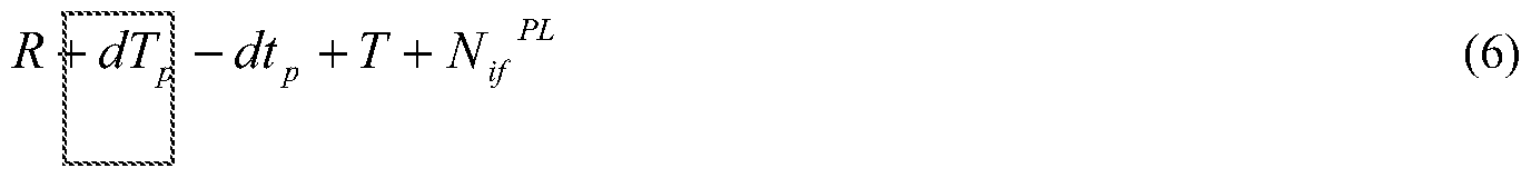
where
dT is a phase-leveled receiver clock (also called a receiver phase clock)
dt is a phase-leveled satellite clock (also called a satellite phase clock)
PL
Nif is a phase-leveled iono-free ambiguity
Satellite phase clock dt in (6) is phase-based and has integer nature and, in contrast to Eq. (4), it can provide phase-leveled ambiguities free of error e , so that: N L = [aNWL ln,eger + βΝ^ ] (7)
PL
The phase-leveled iono-free ambiguity Nif is not an integer but yet has an integer nature; the
pi- phase-leveled iono-free ambiguity Nif can be interpreted as a combination of two integer ambiguities. One way of doing so is assuming that it is a combination of a widelane integer ambiguity
 in which the widelane ambiguity coefficient a and the LI ambiguity coefficient are not necessarily integers.
The phase-leveled clock dt can be quite different from a standard (code-leveled) satellite clock dt . To avoid confusion, the term dt is used to denote the phase-leveled satellite clock and the term dt is used herein to denote the standard (code-leveled) satellite clock, i.e., dt = dt .
The introduction of the phase-leveled satellite clock term dt in (6) means that the corresponding receiver clock term dT is also phase leveled. The term dT is used herein to denote the phase-
Appendix A
leveled receiver clock and the term dTc is used to denote the standard (code-leveled) receiver clock, i.e., dTc = dT . In a positioning engine where phase and code measurements are used simultaneously two clock states are therefore modelled for the receiver; in this formulation these are the phase-leveled receiver clock dT and the standard (code-leveled) receiver clock dTc .
As mentioned above, typical prior-art PPP processing attempts to estimate values for four parameters for each observed satellite: receiver coordinates Xr , Yr ,and Zr , receiver clock dT , tropospheric delay T and the iono-free float ambiguities jf^Floc" _ The introduction of phase- leveled clock terms adds one further parameter to be estimated in the rover engine: phase-leveled receiver clock dT . The restated observation models are therefore as shown in equations (6) and
(2), respectively and reproduced here:

In this formulation each observation type (phase φ or code P ) is corrected with its own clock type (phase-leveled satellite clock dt or code-leveled satellite clock dtc ). Some embodiments of the invention therefore use the phase ψ and code P observations (measurements) of the signals of multiple satellites observed at a rover along with externally-provided code-leveled (standard) satellite clock information dtc and phase-leveled satellite clock information dt to estimate values for range R , code-leveled receiver clock dTc , phase-leveled receiver clock dT ,
PL
tropospheric delay T and the iono-free phase-leveled ambiguities Nif . The state vector of parameters to be estimated in a Kalman-filter implementation, for each satellite j observed at the rover is thus:
Appendix A

PL
Part 12.3 Determining iono-free phase-leveled ambiguities Nif : Option 2
A second formulation for handling the phase-leveled information is to substitute for the code- leveled receiver clock dTc an offset SdTp representing the difference between the code-leveled receiver clock dTc and the phase-leveled receiver clock dTp :
SdTp = dTc - dTp (Π) so that equations (6) and (2) become, respectively:

Accordingly, some embodiments of the invention use the phase φ and code P observations (measurements) of the signals of multiple satellites observed at a rover along with externally- provided code-leveled (standard) satellite clock information dtc and phase-leveled satellite clock information dt to estimate values for range R , phase-leveled receiver clock dT , receiver- clock offset SdTp , tropospheric delay T and the iono-free phase-leveled ambiguities Nif PL .
The state vector of parameters to be estimated in a Kalman-filter implementation, for each satellite j observed at the rover is thus:
Appendix A

This second formulation still has five types of parameters to be estimated, but because δάΤ p is an offset there is less process noise in the Kalman filter than for state vector (10). The advantage of such model as compared to option 1 is that the stochastic model can be setup differently, meaning that the noise level assigned to a clock bias state (e.g. SdTp ) can be different from a clock state
(e.g. dTc ). Assuming that phase- and code-leveled clocks behave in a similar way, the noise level needed for modelling a bias state should be less than for modelling a clock state.
Part 12.4 Determining iono-free phase-leveled ambiguities Nif : Option 3
A third formulation for handling the phase-leveled information is to substitute for the phase- leveled receiver clock dT an offset - dT representing the difference between the phase- leveled receiver clock dT P„ and the code-leveled receiver clock dT L :
- 5dTp = dTp - dTc (15) so that equations (6) and (2) become, respectively:

Accordingly, some embodiments of the invention use the phase φ and code P observations (measurements) of the signals of multiple satellites observed at a rover along with externally-
Appendix A
information dt to estimate values for range R , code-leveled receiver clock dTc , receiver-clock offset - SdTp , tropospheric delay T and the iono-free phase-leveled ambiguities Nif PL . The state vector of parameters to be estimated in a Kalman- filter implementation, for each satellite j observed at the rover is thus:

This third formulation still has five types of parameters to be estimated, but because
offset there is less process noise in the Kalman filter than for state vector (10).
PL
Part 12.5 Determining iono-free phase-leveled ambiguities Nif : Option 4
A fourth formulation for handling the phase-leveled information first estimates the iono-free float
Float
ambiguities Nf- using code-leveled (standard) satellite clocks dtc for phase observations φ
■ Float and for code observations P as in (3), and shifts the iono-free float ambiguities Nf- afterward using the phase-leveled clock information to obtain the iono-free phase-leveled
PL
ambiguities Nif .
The starting point for this formulation is:

Note that (19) and (20) are identical to (lError! Reference source not found.) and (2), since dT. = dT and dt„ = dt .
Appendix A
This fourth formulation, as in the typical prior-art PPP processing discussed above, uses the phase ψ and code P observations (measurements) of the signals of multiple satellites observed at a rover along with externally-provided code-leveled (standard) satellite clock information dtc to estimate values for range R , code-leveled receiver clock dTc , tropospheric delay T and the
Float
iono-free float ambiguities Nif . The state vector of parameters to be estimated in a Kalman- filter implementation, for each satellite j observed at the rover is thus:

As with the prior-art PPP processing, the estimation of parameter values of state vector (21) does
Float
not allow the iono-free float ambiguities Nf- to be reliably determined as iono-free phase-
PL
leveled ambiguities Nif :
Float = N^ PL + e = [ aNwL ^er + Integer ] + g ^ where
Nif is an iono-free float ambiguity representing a combination of a iono-free phase-
PL
leveled ambiguity Nif and an error e
^ integer ^ i(jeiarie integer ambiguity
a is an Widelane ambiguity coefficient
integer ^ ^ integer ambiguity
β is an LI ambiguity coefficient
Appendix A
This fourth formulation assumes that error e represents the difference between the code-leveled (standard) satellite clock dtc and the phase-leveled satellite clock dt :
e = dtc - dt„ (23) so that
[αΝ^'^ + βΝ '^ ] + e - e (25)
[aN^1"'^ + Nl In,eger ] (26)
To summarize, this fourth formulation obtains iono-free float ambiguities Nif a from (19) and then shifts each of these by the difference between the standard (code-leveled) satellite clock dtc J and the phase-leveled clock dtj for the respective satellite j to obtain the iono-free phase-
PL
leveled ambiguities Nif as shown in (24).
For this purpose, the rover can be provided with (1) the standard (code-leveled) satellite clock dtc and the phase-leveled clock dtj for each satellite j observed at the rover, or (2) the standard
(code-leveled) satellite clock dtc 3 and a clock bias <¾c representing the difference between the standard (code-leveled) satellite clock dtj and the phase-leveled clock dt1 , or (3) the phase- leveled clock dtp J and a clock bias dtp representing the difference between the phase-leveled clock dtp J and the standard (code-leveled) satellite clock dtj. . These are equivalent for processing purposes as can be seen from (24).
This fourth formulation has advantages and disadvantages. A disadvantage is that it assumes the behavior of the standard (code-leveled) satellite clock dtc J and the phase-leveled clock dtp J for each satellite j observed at the rover is substantially the same over the period of time for the ambiguity was computed. An advantage is that jumps (integer cycle slips) which might occur in the phase clock estimations can be more easily handled in processing at the rover.
Appendix A
Part 12.6 Determining position using Melbourne-Wuebenna biases b,
After the iono-free phase-leveled ambiguities Nf are determined for a given epoch, they can be single-differenced as VabNjf PL , single-differenced integer (fixed) widelane
afo Integer
ambiguities V NWL can be removed from them to obtain single-differenced LI float ambiguities VabNl , and the single-differenced LI float ambiguities VabNl can be fixed as single-differenced LI integer ambiguities V a Nl
Single-differenced widelane integer ambiguities V NWL are estimated in a widelane- ambiguity filter which runs in parallel with the geometry filter of the rover's processing engine. The rover receiver is provided with a Melbourne-Wuebenna bias b ^ for each of the j satellites in view, e.g., from an external source of data corrections - see Part 7. [WL BIAS PROCESSOR
DESCRIPTION]. Melbourne-Wuebenna bias b ^ can be computed as:
HvL - PNL _ Nj In,e£er , hj hR (Ύ1Λ
~ NWL + bMW ~ bMW \ ι )
is the widelane carrier-phase combination of rover observations of satellite j P^L is the narrowlane code combination of rover observations of satellite j
is the widelane wavelength
Integer
is the widelane integer ambiguity for satellite j
b fjy is the Melbourne-Wuebenna bias for the rover R .
The widelane ambiguity filter eliminates the rover's Melbourne-Wuebenna bias bWL by differencing (27) for each pairing of satellites "a" and "b" to obtain the single-differenced
ab - j Integer
widelane integer ambiguities Vfl¾N, WL
Appendix A

where
Once the single-differenced widelane integer ambiguities V NWL are known, they are removed from the single-differenced iono-free phase-leveled ambiguities Vfli ' Nif PL ' to obtain the single-differenced LI float ambiguities VabNl
PL
The float Kalman filter used to estimate the iono-free phase-leveled ambiguities Nif (or the
Float
iono-free float ambiguities NL in the third alternate formulation discussed above) also gives
CN , the covariance matrix of the iono-free phase-leveled ambiguities Nif . Because the widelane ambiguities are integer (fixed) values after their values are found, CN is the same for

From (7) it is known that:

where
PL
VN^ is the single-difference phase-leveled iono-free ambiguity (differenced between satellites "a" and "b")
VN^ is the single-difference widelane integer ambiguity (differenced between satellites "a" and "b')
afo Float
VN! is the single-difference LI float ambiguity (differenced between satellites "a" and "b")
Therefore
Appendix A
„ Float N, - avNm
VNfl¾ = l-f (31 )
1 β
Because VN^1"'^ are fixed (integer) values, it is assumed that the respective
afo Float
covariance matrices of the LI float ambiguities Nl and the iono-free phase-leveled ambiguities Nl are related by:
C - CNifPl ■ F (32) where
: Float
C Float is the covariance matrix of the LI float ambiguities N,
■ PL
C PL is the covariance matrix of the iono-free phase-leveled ambiguities Nif J
F is a factor to convert the units of the variances from iono-free cycles to LI cycles.
The desired "fixed" (integer-nature) single-differenced LI float ambiguities VN" can be determined from the single-differenced LI float ambiguities VN"* and the covariance matrix afo Float
C T.V., of the LI float ambiguities N, using well-known techniques, such as Lambda
(Jonge et al. 1994), modified Lambda (Chan et al. 2005), weighted averaging of candidate sets, or others. afo Integer
Having determined the single-differenced integer widelane ambiguities VN^ and the single-differenced integer LI ambiguities, integer-nature iono-free ambiguities VN^ are determined from:
 + fNN?Meger
ADDendix A
+ fNN?Meger
ADDendix A
The integer-nature iono-free ambiguities VN are introduced ("pushed") as a pseudo- observation into the Kalman float filter (or optionally a copy of it) to determine a rover position based on integer-nature ambiguities. The state vector of the float filter copy is thus:

The rover position can then be determined with an accuracy (and precision) substantially better than for the typical prior-art PPP processing in which the ambiguities are considered to be float numbers, as shown in FIG. [47]
Part 12.7 Ambiguity Fixing References
Jonge de, P. J., and C.C.J.M. Tiberius (1994). A new GPS ambiguity estimation method based on integer least squares. Proceedings of the 3rd International Symposium on Differential Satellite Navigation Systems DSNS'94, London, UK, April 18-22, Paper No. 73, 9 pp.
X. -W. Chang, X. Yang and T. Zhou (2005). MLAMBDA: a modified LAMBDA method for integer least-squares estimation. Journal of Geodesy, Springer Berlin / Heidelberg. Volume 79, Number 9 / December, 2005, pp.552-565.
Appendix A
Part 13: Summary of Some of the Inventive Concepts
Section 13A: MW (Melbourne- Wiibbena) Bias Processing (A-2565)
[BR Note: Abstract (FIG. 8A)]
[MW Processing] A method of processing a set of GNSS signal data derived from code observations and carrier-phase observations at multiple receivers of GNSS signals of multiple satellites over multiple epochs, the GNSS signals having at least two carrier frequencies, comprising:
a. forming an MW (Melbourne-Wiibbena) combination per receiver-satellite
pairing at each epoch to obtain a MW data set per epoch,
b. estimating from the MW data set per epoch an MW bias per satellite which may vary from epoch to epoch, and a set of WL (widelane) ambiguities, each WL ambiguity corresponding to one of a receiver-satellite link and a satellite- receiver-satellite link, wherein the MW bias per satellite is modeled as one of (i) a single estimation parameter and (ii) an estimated offset plus harmonic variations with estimated amplitudes.
The method of 1, further comprising applying corrections to the GNSS signal data. The method of one of 1-2, further comprising smoothing at least one linear combination of GNSS signal data before estimating a MW bias per satellite.
The method of one of 1-3, further comprising applying at least one MW bias constraint.
The method of one of 1-4, further comprising applying at least one integer WL ambiguity constraint
The method of one of 1 -4, further comprising using a spanning tree (ST) over one of an observation graph and a filter graph for constraining the WL ambiguities.
The method of one of 1 -4, further comprising using a minimum spanning tree (MST) on one of an observation graph and a filter graph for constraining the WL ambiguities.
The method of 7, wherein the minimum spanning tree is based on edge weights, each edge weight derived from receiver-satellite geometry.
Appendix A
The method of 8, wherein the edge weight is defined with respect to one of (i) a geometric distance from receiver to satellite, (ii) a satellite elevation angle, and (iii) a geometric distance from satellite to receiver to satellite, and (iv) a combination of the elevations under which the two satellites in a single differenced combination are seen at a station.
The method of 7, wherein the minimum spanning tree is based on edge weights, with each edge weight based on WL ambiguity information, defined with respect to one of (i) difference of a WL ambiguity to integer, (ii) WL ambiguity variance, and (iii) a combination of (i) and (ii).
The method of one of 1-10, further comprising fixing at least one of the WL ambiguities as an integer value.
The method of one of 1-10, further comprising determining candidate sets of WL integer ambiguity values, forming a weighted combination of the candidate sets, and fixing at least one of the WL ambiguities as a value taken from the weighted combination.
The method of one of 11-12, wherein the estimating step comprises introducing fixed WL ambiguities so as to estimate MW biases which are compatible with fixed WL ambiguities.
The method of 13 wherein the estimating step comprises applying an iterative filter to the MW data per epoch and wherein introducing fixed WL ambiguities comprises one of (i) putting the fixed WL ambiguities as observations into the filter, (ii) putting the fixed WL ambiguities as observations into a copy of the filter generated after each of a plurality of observation updates, and (iii) reducing the MW combinations by the fixed WL ambiguities and putting the resulting reduced MW combinations into a second filter without ambiguity states to estimate at least one MW bias per satellite.
The method of one of 1-14, further comprising shifting at least one MW bias by an integer number of WL cycles.
The method of one of 1-14, further comprising shifting at least one MW bias and its respective WL ambiguity by an integer number of WL cycles.
The method of one of 1-16 wherein the navigation message comprises orbit information,
Apparatus for perform the method of one of 1 - 17.
Appendix A
A computer program comprising instructions configured, when executed on a computer processing unit, to carry out a method according to one of 1 - 17. A computer-readable medium comprising a computer program according to 19.
ADDendix A
Section 13B: Orbit Processing (A-2647)
[BR Note: Abstract (FIG. 26B)]
A method of processing a set of GNSS signal data derived from signals of GNSS satellites observed at reference station receivers, the data representing code observations and carrier observations on each of at least two carriers over multiple epochs, comprising: a. obtaining an orbit start vector (2635) comprising: a time sequence of predicted positions and predicted velocities for each satellite over a first interval [of multiple epochs], and the partial derivatives of the predicted positions and predicted velocities with respect to initial positions, initial velocities, [other] force model parameters and Earth orientation parameters,
b. obtaining ionospheric-free linear combinations (2645) of the code observations and the carrier observations for each satellite at multiple reference stations, and c. iteratively correcting the orbit start vector (2635) using a time sequence of the ionospheric-free linear combinations (2645) and predicted Earth orientation parameters (2610) to obtain an updated orbit start vector values (2680) comprising a time sequence of predicted positions and predicted velocities for each satellite over a subsequent interval of epochs and an estimate of Earth orientation parameters.
[Startup] The method of 1, wherein obtaining an orbit start vector (2635) comprises:
i. obtaining an approximate orbit vector (2615) for the satellites, ii. obtaining predicted Earth orbit parameters (2610),
iii. iteratively integrating the approximate orbit vector with the predicted Earth orbit parameters to obtain an orbit prediction (2620) for an initial time interval and, with each iteration, adapting the orbit prediction (2620) to the approximate orbit vector, and
iv. preparing from the orbit prediction (2620) an initial set of values for the orbit start vector and partial derivatives (2635).
The method of 2, wherein the approximate orbit vector (2615) is obtained from one of: a broadcast satellite navigation message, IGS Ultra-rapid Orbits data, and another source of predicted orbits.
Appendix A
The method of one of 2 - 3, wherein adapting the orbit prediction (2620) to the approximate orbit vector (2615) is performed using a least squares approach.
The method of one of 2 - 4, wherein integrating the approximate orbit vector (2615) with the predicted Earth orientation parameters (2610) to obtain an orbit prediction (2620) is iterated until the orbit prediction remains substantially constant.
The method of 1, wherein obtaining an orbit start vector (2635) comprises preparing the orbit start vector (2635) from a set of the updated orbit start vector values (2680) which is not older than a predetermined time interval.
The method of 6, wherein the predetermined time interval is not more than a few hours. [Operation] The method of one of 6 - 7, wherein preparing the orbit start vector (2635) comprises: mapping a new orbit start vector (2690) from the updated orbit start vector (2680) and integrating the new orbit start vector (2690) to obtain new values for the orbit start vector (2635).
The method of 8, wherein integrating the new orbit start vector (2690) comprises integrating the new orbit start vector using Earth orientation parameters from the updated start vector values 2680.
[Kalman] The method of one of 1 - 9, wherein correcting comprises applying an iterative filter comprising one of: a Kalman filter, a UD factorized filter, and a Square Root Information Filter.
[Satellite parameters] The method of one of 1 - 10, wherein the updated orbit state vector (2680) further comprises estimating additional parameters for each satellite, and wherein correcting the orbit start vector comprises correcting the additional parameters for each satellite.
[Output] The method of one of 1 - 11, further comprising: mapping values from the updated orbit start vector 2680 to a current epoch to obtain a current-epoch orbit position and velocity for each satellite.
[Fixing] The method of one of 1 - 6, wherein the state vector further comprises an ionospheric-free ambiguity (2575) per receiver-satellite pair, and correcting the orbit start vector (2635) comprises estimating float values for the ionospheric-free ambiguities, and wherein the method further comprises:
1. obtaining a value for a widelane ambiguity (340) per receiver- satellite pair, the widelane ambiguity values having integer nature,
Appendix A
2. determining integer-nature values for ambiguities linearly related to the widelane ambiguities and the ionospheric-free ambiguities from the values of the widelane ambiguities and the float values of the ionospheric-free ambiguities,
3. fixing the values of the ionospheric-free ambiguities using the integer-nature values,
4. with the values of the ionospheric-free ambiguities fixed,
iteratively correcting the orbit start vector (2635) using a time sequence of the ionospheric-free linear combinations (2645) and a set of Earth orbit parameters to obtain an updated orbit start vector (2680) comprising a time sequence of predicted positions and predicted velocities for each satellite over an interval of multiple epochs and an estimate of Earth orientation parameters.
14. The method of 13, wherein the ambiguities linearly related to the widelane ambiguities and the ionospheric-free ambiguities comprise one of: narrowlane ambiguities, LI ambiguities and L2 ambiguities.
15. [Epoch] The method of one of 1 - 14, wherein the epochs occur at a rate of about 1 Hz.
16. [Filter Update] The method of one of 1 - 15, wherein iteratively correcting the orbit start vector comprises estimating for each epoch the values of a satellite clock for each satellite and a satellite position for each satellite at each epoch.
17. [Filter Update] The method of one of 1 - 15, wherein iteratively correcting the orbit start vector comprises estimating for each epoch the values of a satellite clock for each satellite, a satellite clock drift, a satellite clock drift rate, and a satellite position for each satellite at each epoch.
18. [Orbit Estimate] The method of one of 1 - 17, wherein the predicted time sequence of approximate positions for each satellite for at least some of the epochs covers an interval of at least 150 seconds.
19. [Worldwide network] The method of one of 1 - 18, wherein the reference stations are widely distributed about the Earth and the GNSS signal data from each reference station represents code observations and carrier observations of a subset of the GNSS satellites at each epoch.
20. Apparatus adapted to perform the method of one of 1 - 19.
Appendix A
A computer program comprising instructions configured, when executed on a computer processing unit, to carry out a method according to one of 1 - 19.
A computer-readable medium comprising a computer program according to 21.
Appendix A
Section 13C: Phase Clock Processing (A-2585)
[BR Note: Abstract (FIG. 27)]
[Estimating Phase Clocks] Network Processing - Phase Clocks] A method of processing a set of GNSS signal data derived from code observations and carrier-phase observations at multiple receivers of GNSS signals of multiple satellites over multiple epochs, the GNSS signals having at least two carrier frequencies and a navigation message containing orbit information, comprising:
a. obtaining precise orbit information for each satellite,
b. determining at least one set of ambiguities per receiver, each ambiguity
corresponding to one of a receiver-satellite link and a satellite-receiver-satellite link, and
c. using at least the precise orbit information, the ambiguities and the GNSS signal data to estimate a phase-leveled clock per satellite.
The method of 1, wherein determining ambiguities is performed at a first rate and wherein estimating a phase-leveled clock per satellite is performed at a second rate higher than the first rate.
The method of one of 1-2, wherein estimating the phase-leveled clock per satellite comprises:
i. using at least the precise orbit information, the ambiguities and the
GNSS singal data to estimate a set of phase-leveled clocks per receiver, each phase-leveled clock corresponding to one of a receiver-satellite link and a satellite-receiver-satellite link, and
ii. using a pluraility of the phase-leveled clocks to estimate one phase- leveled clock per satellite.
The method of one of 1 - 3, wherein determining the ambiguities comprises using at least one phase-leveled clock per satellite previously estimated to estimate the ambiguities. The method of one of 4, further comprising obtaining at least one additional phase- leveled clock per satellite estimated from an external source, and wherein determining the ambiguities comprises using said at least one additional phase-leveled clock per satellite to estimate the ambiguities.
The method of one of 1-5, further comprising
Annsndix A
1. determining at least one set of ambiguities per receiver for
additional receivers, each ambiguity corresponding to one of a receiver-satellite link and a satellite-receiver-satellite link,
2. after determining the ambiguities for the additional receivers, using at least the precise orbit information, the ambiguities for the additional receivers and the GNSS signal data to estimate the at least one additional phase-leveled clock per satellite
The method of one of 1 - 6, wherein the at least two carrier frequencies comprise at least two of the GPS LI, GPS L2 and GPS L5 frequencies.
The method of one of 1 - 7, wherein determining at least one set of ambiguities per receiver comprises at least one of: estimating float ambiguity values, estimating float ambiguity values and fixing the float ambiguity values to integer values, estimating float ambiguity values and forming at least one weighted average of integer value candidates, and constraining the ambiguity values in a sequential filter.
The method of one of 1 - 8, wherein the ambiguities are undifferenced between satellites. The method of one of 1 - 8, wherein the ambiguities are single-differenced between satellites.
Apparatus adapted to perform the method of one of 1-10.
A computer program comprising instructions configured, when executed on a computer processing unit, to carry out a method according to one of 1 - 10.
A computer-readable medium comprising a computer program according to 12.
Appendix A
Section 13D: Rover Processing with Synthesized Reference Station Data (A-2617) [BR Note: Abstract (FIG. 38) [SBS Processing] A method of determining position of a rover antenna, comprising: a. obtaining rover GNSS data derived from code observations and carrier phase observations of GNSS signals of multiple satellites over multiple epochs, b. obtaining precise satellite data for the satellites,
c. determining a virtual base station location,
d. generating epochs of synthesized base station data using at least the precise satellite data and the virtual base station location,
e. applying a differential process to at least the rover GNSS data and the
synthesized base station data to determine at least rover antenna positions.
[Low Latency] The method of 1, wherein generating epochs of synthesized base station data comprises generating an epoch of virtual base station data for each epoch of GNSS rover data.
[High Accuracy] The method of 1, wherein obtaining precise satellite data comprises obtaining precise satellite data in sets, wherein generating epochs of synthesized base station data comprises generating an epoch of synthesized base station data for each set of precise satellite data, and wherein applying a differential process comprises matching each set of GNSS rover data with an epoch of synthesized base station data.
[Virtual Base Station Location] The method of one of 1 - 3, wherein determining a virtual base station location comprises determining the virtual base station location from at least one of: an autonomously determined position of the rover antenna, a previously determined one of said rover antenna positions, a synthesized base station data generating module, an inertial navigation system, a mobile telephone tower location, and information provided by a user.
The method of one of 1 - 4, further comprising updating the virtual base station location on the occurrence of at least one of: never, for each epoch of rover data, when the distance between an approximate rover antenna position and the virtual base station location exceeds a predetermined threshold, and for each update of the rover antenna positions.
Appendix A
The method of one of 1 - 5, wherein each epoch of the synthesized base station data is generated for a corresponding virtual base station location.
The method of one of 1 - 5, wherein determining the virtual base station location comprises selecting a virtual base station location close to a current approximate rover antenna position.
The method of one of 1 - 7, wherein a new virtual base position is determined when one or more of the following criteria is met: each rover epoch, each nth rover epoch, after a time interval, after exceeding a distance between a current approximate rover position and a current virtual base station location.
The method of one of 1 - 8, wherein the virtual base station location is generated for a specific GNSS time interval
The method of one of 1 - 9, wherein applying a differential process to at least the rover GNSS data and the synthesized base station data to determine at least rover antenna positions comprises at least one of:: aided ins (integrated ins, gnss processing); normal rtk; irtk; dgps; float; triple differenced; post processed or realtime.
The method of one of 1 - 10, further comprising matching each epoch of the rover GNSS data with an epoch of synthesized base station data within a few milliseconds.
The method of one of 1 - 11, wherein generating epochs of synthesized base station data comprises a set of synthesized base station observations for each of a plurality of discrete times, and wherein applying a differential process comprises processing each epoch of GNSS rover data with a set of synthesized base station observations for a discrete time which is within ten seconds of the epoch of the GNSS rover data being processed. Apparatus adapted to perform the method of one of 1-12.
A computer program comprising instructions configured, when executed on a computer processing unit, to carry out a method according to one of 1 - 12.
A computer-readable medium comprising a computer program according to 14.
Appendix A
Section 13E: Rover Processing with Ambiguity Fixing (A-2599)
[BR Note: Abstract (FIG. 49)]
[Draft claims to be revised]
TNL A-2599 Ambiguity Fixing
1. A method of processing a set of GNSS signal data derived from signals of a set of satellites having carriers observed at a rover antenna, wherein the data includes a carrier observation and a code observation of each carrier of each satellite, comprising:
a. obtaining for each satellite clock corrections comprising at least two of: (i) a code-leveled satellite clock, (ii) a phase-leveled satellite clock, and (iii) a satellite clock bias representing a difference between a code-leveled satellite clock and a phase-leveled satellite clock,
b. running a first filter which uses at least the GNSS signal data and the satellite clock corrections to estimate values for parameters comprising at least one carrier ambiguity for each satellite, and a covariance matrix of the carrier ambiguities, c. determining from each carrier ambiguity an integer-nature carrier ambiguity comprising one of: an integer value, and a combination of integer candidates, d. inserting the integer-nature carrier ambiguities as pseudo-observations into a second filter, and applying the second filter to the GNSS signal data and the satellite clock corrections to obtain estimated values for parameters comprising at least the position of the receiver.
2. The method of 1, wherein the integer-nature carrier ambiguities are between-satellite single-differenced ambiguities.
3. The method of one of 1 - 2, further comprising
a. obtaining a set of MW corrections,
b. running a third filter using the GNSS signal data and at least the MW corrections to obtain at least a set of WL ambiguities,
c. using the set of WL ambiguities to obtain the integer-nature carrier ambiguity.
4. The method of 3, wherein the WL ambiguities comprise at least one of: float values, integer values, and float values based on integer candidates.
Appendix A
The method of 4, wherein the covariance matrix of the ambiguities is scaled to reflect the change due to the use of the WL ambiguities.
The method of one of 1 - 5, wherein the WL ambiguties are between-satellite single- differenced ambiguities.
The method of one of 1 - 6, wherein the integer-nature ambiguities comprise at least one of: L1-L2 ionospheric-free ambiguities, L2-L5 ionospheric-free ambiguities, and carrier ambiguities of a linear combination of two or more GNSS frequencies.
The method of one of 1 - 6, wherein ionospheric delay information isused to fee one or more of the filters and wherein the integer-nature ambiguity comprises at least one of: carrier ambiguity of LI frequency, carrier ambiguity of L2 frequency, carrier ambiguity of L5 frequency, and carrier ambiguity of any GNSS frequency.
The method of one of 1 - 8, wherein the second filter comprises: a new filter, a copy of the first filter, and the first filter.
The method of one of 1 - 9, where the code-leveled satellite clock is used for modeling all GNSS observations, and the float ambiguity is adapted to the level of the phase-leveled clock by applying the difference between the code-leveled satellite clock and the phase-leveled satellite clock.
The method of one of 1 - 9, wherein the code-leveled clock is used for modeling all GNSS code observations and the phase-leveled clock is used for modeling all GNSS carrier observations.
The method of one of 1 - 11 , wherein determining the integer-nature carrier ambiguity from a float ambiguity comprise at least one of: rounding the float ambiguity to the nearest integer, choosing best integer candidates from a set of integer candidates generated using integer least squares, and computing float values using a set of integer candidates generated using integer least squares.
The method of one of 1 -12, wherein at least one of the first filter and third filter further estimates at least one of: receiver phase-leveled clock, receiver code-leveled clock, tropospheric delay, receiver clock bias representing a difference between the code-leveled receiver clock and the phase-leveled receiver clock, and multipath states.
The method of one of 1 -13, wherein at least one of the first filter, the second filter and the third filter is adapted ot update the estimated values for each of a plurality of epochs of GNSS signal data.
Appendix A
Apparatus adapted to perform the method of one of 1-14.
A computer program comprising instructions configured, when executed on a computer processing unit, to carry out a method according to one of 1 - 14. A computer-readable medium comprising a computer program according to 16.
Appendix A
Any plurality of the above described aspects of the invention may be combined to form further aspects and embodiments, with the aim of providing additional benefits notably in terms of surveying efficiency and/or system usability.
Above-described methods, apparatuses and their embodiments may be integrated into a rover, a reference receiver or a network station, and/or the processing methods described can be carried out in a processor which is separate from and even remote from the receiver/s used to collect the observations (e.g., observation data collected by one or more receivers can be retrieved from storage for post-processing, or observations from multiple network reference stations can be transferred to a network processor for near-real-time processing to generate a correction data stream and/or virtual-reference-station messages which can be transmitted to one or more rovers). Therefore, the invention also relates to a rover, a reference receiver or a network station including any one of the above apparatuses.
In some embodiments, the receiver of the apparatus of any one of the above-described embodiments is separate from the filter and the processing element. Post-processing and network processing of the observations may notably be performed. That is, the constituent elements of the apparatus for processing of observations does not itself require a receiver. The receiver may be separate from and even owned/operated by a different person or entity than the entity which is performing the processing. For postprocessing, the observations may be retrieved from a set of data which was previously collected and stored, and processed with reference-station data which was previously collected and stored; the processing is conducted for example in an office computer long after the data collection and is thus not real-time. For network processing, multiple reference-station receivers collect observations of the signals from multiple satellites, and this data is supplied to a network processor which may for example generate a correction data stream or which may for example generate a "virtual reference station" correction which is supplied to a rover so that the rover can perform differential processing. The
ADDendix A
data provided to the rover may be ambiguities determined in the network processor, which the rover may use to speed its position solution, or may be in the form of corrections which the rover applies to improve its position solution. The network is typically operated as a service to rover operators, while the network operator is typically a different entity than the rover operator.
Any of the above-described methods and their embodiments may be implemented by means of a computer program. The computer program may be loaded on an apparatus, a rover, a reference receiver or a network station as described above. Therefore, the invention also relates to a computer program, which, when carried out on an apparatus, a rover, a reference receiver or a network station as described above, carries out any one of the above above-described methods and their embodiments.
The invention also relates to a computer-readable medium or a computer-program product including the above-mentioned computer program. The computer-readable medium or computer-program product may for instance be a magnetic tape, an optical memory disk, a magnetic disk, a magneto-optical disk, a CD ROM, a DVD, a CD, a flash memory unit or the like, wherein the computer program is permanently or temporarily stored. The invention also relates to a computer-readable medium (or to a computer- program product) having computer-executable instructions for carrying out any one of the methods of the invention.
The invention also relates to a firmware update adapted to be installed on receivers already in the field, i.e. a computer program which is delivered to the field as a computer program product. This applies to each of the above-described methods and apparatuses.
GNSS receivers may include an antenna, configured to received the signals at the frequencies broadcasted by the satellites, processor units, one or more accurate clocks
ADDendix A
(such as crystal oscillators), one or more computer processing units (CPU), one or more memory units (RAM, ROM, flash memory, or the like), and a display for displaying position information to a user.
Where the terms "receiver", "filter" and "processing element" are used herein as units of an apparatus, no restriction is made regarding how distributed the constituent parts of a unit may be. That is, the constituent parts of a unit may be distributed in different software or hardware components or devices for bringing about the intended function. Furthermore, the units may be gathered together for performing their functions by means of a combined, single unit. For instance, the receiver, the filter and the processing element may be combined to form a single unit, to perform the combined functionalities of the units.
The above-mentioned units may be implemented using hardware, software, a combination of hardware and software, pre-programmed ASICs (application-specific integrated circuit), etc. A unit may include a computer processing unit (CPU), a storage unit, input/output (I/O) units, network connection units, etc.
Although the present invention has been described on the basis of detailed examples, the detailed examples only serve to provide the skilled person with a better understanding, and are not intended to limit the scope of the invention. The scope of the invention is much rather defined by the appended claims.
Claims
1. A positioning method, comprising:
a. obtaining GNSS data derived from signals received at a rover antenna, b. obtaining at least one of correction data and rigorous satellite data, c. maintaining a time sequence of at least one rover position and at least one rover position difference with associated time tags,
d. using the time sequence to determine at least one derived rover position, e. reporting the derived rover position, and
f. maintaining a set of GNSS satellite clock error models, comprising i. upon arrival of rover data associated with a new time tag, extending the time sequence, and
ii. upon arrival of rigorous satellite data, updating at least one clock error model.
2. The method of claim 1, wherein maintaining a set of GNSS satellite clock error
models further comprises, upon arrival of rigorous satellite orbit and clock data, updating the time sequence.
3. The method of claim 1, further comprising using the updated at least one clock error model to update at least one rover position of the time sequence.
4. The method of claim 1, wherein the set of satellite clock error models comprises up to one clock error model per satellite.
5. The method of claim 1, wherein the correction data comprises at least one of: single- base-station observations, virtual reference station observations derived from reference stations of a regional network, synthetic base station observations derived from reference stations of a global network, synthetic reference station observations derived from reference stations of a global network with regional augmentation, and state space representations.
6. The method of claim 1, wherein rigorous satellite data comprises precise orbit and precise clock data per satellite.
7. Positioning apparatus comprising a processor and memory and a set of instructions enabling the processor to:
a. obtain GNSS data derived from signals received at a rover antenna,
INTERNATIONAL APPLICATION FOR PATENT PCT/US2012/029694 b. obtain at least one of correction data and rigorous satellite data,
c. maintain a time sequence of at least one rover position and at least one rover position difference with associated time tags,
d. use the time sequence to determine at least one derived rover position, e. report the derived rover position, and
f. maintain a set of GNSS satellite clock error models by
i. upon arrival of rover data associated with a new time tag, extending the time sequence, and
ii. upon arrival of rigorous satellite data, updating at least one clock error model.
8. The apparatus of claim 7, further comprising instructions enabling the processor to update the time sequence upon arrival of rigorous satellite orbit and clock data.
9. The apparatus of claim 7, further comprising instructions enabling the processor to update at least one rover position of the time sequence using the updated at least one clock error model.
10. The apparatus of claim 7, wherein the set of satellite clock error models comprises up to one clock error model per satellite.
1 1. The apparatus of claim 7, wherein the correction data comprises at least one of:
single-base-station observations, virtual reference station observations derived from reference stations of a regional network, synthetic base station observations derived from reference stations of a global network, synthetic reference station observations derived from reference stations of a global network with regional augmentation, and state space representations.
12. The apparatus of claim 7, wherein rigorous satellite data comprises precise orbit and precise clock data per satellite.
13. A computer program product comprising a tangible computer-readable medium
embodying instructions for causing an apparatus to perform the method of claim 1.
14. A computer program comprising instructions for causing an apparatus to perform the method of claim 1.
INTERNATIONAL APPLICATION FOR PATENT PCT/US2012/029694
[Part B: Mixed Delta - mixing quality in one epoch] [TNL A-2798]
15. A positioning method, comprising
a. obtaining GNSS data derived from signals received at a rover antenna, b. obtaining at least one of correction data and rigorous satellite data, c. maintaining a time sequence of at least one rover position and at least one rover position difference with associated time tags, by estimating at least one position difference using rigorous satellite data from multiple satellites using at least two selected combinations of
i. for at least one satellite, no correction data and broadcast satellite data,
ii. for at least one satellite, no correction data and rigorous predicted satellite data,
iii. for at least one satellite, no correction data rigorous satellite data for said at least one satellite,
iv. for at least one satellite, correction data and broadcast satellite data, v. for at least one satellite, rigorous predicted satellite data and
correction data,
vi. for at least one satellite, rigorous satellite data and correction data, d. using the time sequence to determine at least one derived rover position, and e. reporting the derived rover position.
16. The method of claim 15, wherein estimating at least one position difference using rigorous satellite data from multiple satellites using at least two selected
combinations comprises applying a filter having two clock states per satellite.
17. The method of claim 15, wherein the correction data comprises at least one of: single- base-station observations, virtual reference station observations derived from reference stations of a regional network, synthetic base station observations derived from reference stations of a global network, synthetic reference station observations derived from reference stations of a global network with regional augmentation, and state space representations.
18. The method of claim 15, wherein rigorous satellite data comprises rigorous orbit data per satellite and rigorous clock data per satellite.
19. Positioning apparatus comprising a processor and memory and a set of instructions enabling the processor to:
2012/151006 INTERNATIONAL APPLICATION FOR PATENT PCT/US2o12/029694 a. obtain GNSS data derived from signals received at a rover antenna, b. obtain at least one of correction data and rigorous satellite data,
c. maintain a time sequence of at least one rover position and at least one rover position difference with associated time tags, by estimating at least one position difference using rigorous satellite data from multiple satellites using at least two selected combinations of
i. for at least one satellite, no correction data and broadcast satellite data,
ii. for at least one satellite, no correction data and rigorous predicted satellite data,
iii. for at least one satellite, no correction data rigorous satellite data for said at least one satellite,
iv. for at least one satellite, correction data and broadcast satellite data, v. for at least one satellite, rigorous predicted satellite data and
correction data,
vi. for at least one satellite, rigorous satellite data and correction data, d. use the time sequence to determine at least one derived rover position, and e. report the derived rover position.
20. The apparatus of claim 19, further comprsing a filter having two clock states per
satellite, wherein the filter is adapted to estimate at least one position difference using rigorous satellite data from multiple satellites using at least two selected
combinations.
21. The apparatus of claim 19, wherein the correction data comprises at least one of: single-base-station observations, virtual reference station observations derived from reference stations of a regional network, synthetic base station observations derived from reference stations of a global network, synthetic reference station observations derived from reference stations of a global network with regional augmentation, and state space representations.
22. The apparatus of claim 19, wherein rigorous satellite data comprises rigorous orbit data per satellite and rigorous clock data per satellite.
23. A computer program product comprising a tangible computer-readable medium
embodying instructions for causing an apparatus to perform the method of claim 15.
2012/151006 INTERNATIONAL APPLICATION FOR PATENT PCT/US2o12/029694
24. A computer program comprising instructions for causing an apparatus to perform the method of claim 15.
O 2012/151006 INTERNATIONAL APPLICATION FOR PATENT PCT/US2o12/029694
[Part C: Improve/cleanup the buffer] [TNL A-3126]
25. A positioning method, comprising
a. obtaining GNSS data derived from signals received at a rover antenna, b. obtaining at least one of correction data and rigorous satellite data, c. maintaining a time sequence of at least one rover position and at least one rover position difference with associated time tags by,
i. upon arrival of correction data, extending the time sequence with a computed synchronized position, and
ii. upon arrival of one of correction data and rigorous satellite data, modifying at least a portion of the time sequence,
d. using the time sequence to determine at least one derived rover position, and e. reporting the derived rover position.
26. The method of claim 25, wherein the computed synchronized position comprises one of: a real-time kinematic position, a position determined using a weighted average of integer ambiguity candidates, a position determined using a differential positioning technique, a position determined with the aid of an inertial navigation system, and a technique using GNSS data to determine an absolute position.
27. The method of claim 25, wherein modifying at least a portion of the time sequence comprises replacing at least one position difference by at least one improved position difference.
28. The method of claim 27, wherein replacing at least one position difference by at least one improved position difference comprises replacing at least one position difference determined using broadcast satellite data with at least one position difference determined using rigorous predicted satellite data.
29. The method of claim 27, wherein replacing at least one position difference by at least one improved position difference comprises blending at least one position difference determined using broadcast satellite data with at least one position difference determined using rigorous predicted satellite data.
30. The method of claim 27, wherein replacing at least one position difference by at least one improved position difference comprises replacing at least one position difference determined using rigorous predicted satellite data with at least one position difference determined using rigorous satellite data.
INTERNATIONAL APPLICATION FOR PATENT PCT/US2012/029694
31. The method of claim 27, wherein replacing at least one position difference by at least one improved position difference comprises blending at least one position difference determined using rigorous predicted satellite data with at least one position difference determined using rigorous satellite data.
32. The method of claim 27, wherein replacing at least one position difference by at least one improved position difference comprises replacing at least one position difference determined using rigorous satellite data with at least one position difference determined using corrected single-differenced data.
33. The method claim 27, wherein replacing at least one position difference by at least one improved position difference comprises blending at least one position difference determined using rigorous satellite data with at least one position difference determined using corrected single-differenced data.
34. The method of claim 27, wherein replacing at least one position difference by at least one improved position difference comprises replacing at least one position difference determined using corrected single-differenced data with at least one position difference determined using corrections synchronous with rover data.
35. The method of claim 27, wherein replacing at least one position difference by at least one improved position difference comprises blending at least one position difference determined using corrected single-differenced data with at least one position difference determined using corrections synchronous with rover data.
36. The method of claim 25, wherein maintaining a time sequence further comprises, upon arrival of rigorous satellite data, replacing at least one position difference by at least one improved position difference.
37. The method of claim 25, wherein modifying at least a portion of the time sequence comprises replacing a portion of the time sequence with an improved portion of the time sequence.
38. The method of claim 37, wherein the improved portion of the time sequence has an estimated precision which is better than an estimated precision of a portion of the time sequence which it replaces.
39. The method of claim 37, wherein the improved portion of the time sequence has a number of entries which is fewer than a number of entries of a portion of the time sequence which it replaces.
INTERNATIONAL APPLICATION FOR PATENT PCT/US2012/029694
40. The method of claim 37, wherein the improved portion of the time sequence is
determined by, starting from a position determined using corrections synchronous with rover data as an anchor position at a time tag, deriving a new anchor position for the time tag from the anchor position and at least one other previously estimated position at the time tag.
41. The method of claim 40, wherein deriving a new anchor position for the time tag
comprises selecting between the anchor position and the at least one other previously estimated position at the time tag based on comparison of an estimated precision of the anchor position with an estimated precision of the at least one other previously estimated position at the time tag.
42. The method of claim 41, wherein at least one estimated precision is determined from a covariance matrix.
43. The method of claim 41, wherein the new anchor position for the time tag is selected based on smallest estimated three-dimensional precision.
44. The method of claim 41, wherein the new anchor position for the time tag is selected based on smallest estimated horizontal precision.
45. The method of claim 41, wherein the new anchor position for the time tag is selected based on smallest vertical precision.
46. The method of claim 40, wherein deriving a new anchor position for the time tag
comprises blending the anchor position with the at least one other previously estimated position at the time tag.
47. The method of claim 46, wherein blending comprises forming a weighted mean of the anchor position and at least one other previously estimated position at the time tag.
48. Positioning apparatus comprising a processor and memory and a set of instructions enabling the processor to:
a. obtain GNSS data derived from signals received at a rover antenna, b. obtain at least one of correction data and rigorous satellite data,
c. maintain a time sequence of at least one rover position and at least one rover position difference with associated time tags by,
i. upon arrival of correction data, extending the time sequence with a computed synchronized position, and
ii. upon arrival of one of correction data and rigorous satellite data, modifying at least a portion of the time sequence,
INTERNATIONAL APPLICATION FOR PATENT PCT/US2012/029694 d. use the time sequence to determine at least one derived rover position, and e. report the derived rover position.
49. The apparatus of claim 48, wherein the computed synchronized position comprises one of: a real-time kinematic position, a position determined using a weighted average of integer ambiguity candidates, a position determined using a differential positioning technique, a position determined with the aid of an inertial navigation system, and a technique using GNSS data to determine an absolute position.
50. The apparatus of claim 48, wherein modifying at least a portion of the time sequence comprises replacing at least one position difference by at least one improved position difference.
51. The apparatus of claim 48, wherein replacing at least one position difference by at least one improved position difference comprises replacing at least one position difference determined using broadcast satellite data with at least one position difference determined using rigorous predicted satellite data.
52. The apparatus of claim 51, wherein replacing at least one position difference by at least one improved position difference comprises blending at least one position difference determined using broadcast satellite data with at least one position difference determined using rigorous predicted satellite data.
53. The apparatus of claim 51, wherein replacing at least one position difference by at least one improved position difference comprises replacing at least one position difference determined using rigorous predicted satellite data with at least one position difference determined using rigorous satellite data.
54. The apparatus of claim 51, wherein replacing at least one position difference by at least one improved position difference comprises blending at least one position difference determined using rigorous predicted satellite data with at least one position difference determined using rigorous satellite data.
55. The apparatus of claim 51, wherein replacing at least one position difference by at least one improved position difference comprises replacing at least one position difference determined using rigorous satellite data with at least one position difference determined using corrected single-differenced data.
56. The apparatus of claim 51, wherein replacing at least one position difference by at least one improved position difference comprises blending at least one position
INTERNATIONAL APPLICATION FOR PATENT PCT/US2012/029694 difference determined using rigorous satellite data with at least one position difference determined using corrected single-differenced data.
57. The apparatus of claim 51, wherein replacing at least one position difference by at least one improved position difference comprises replacing at least one position difference determined using corrected single-differenced data with at least one position difference determined using corrections synchronous with rover data.
58. The apparatus of claim 51, wherein replacing at least one position difference by at least one improved position difference comprises blending at least one position difference determined using corrected single-differenced data with at least one position difference determined using corrections synchronous with rover data.
59. The apparatus of claim 48, wherein to maintain a time sequence further comprises, upon arrival of rigorous satellite data, to replace at least one position difference by at least one improved position difference.
60. The apparatus of claim 51, wherein modifying at least a portion of the time sequence comprises replacing a portion of the time sequence with an improved portion of the time sequence.
61. The apparatus of claim 60, wherein the improved portion of the time sequence has an estimated precision which is better than an estimated precision of a portion of the time sequence which it replaces.
62. The apparatus of claim 60, wherein the improved portion of the time sequence has a number of entries which is fewer than a number of entries of a portion of the time sequence which it replaces.
63. The apparatus of claim 60, wherein the improved portion of the time sequence is
determined by, starting from a position determined using corrections synchronous with rover data as an anchor position at a time tag, deriving a new anchor position for the time tag from the anchor position and at least one other previously estimated position at the time tag.
64. The apparatus of claim 63, wherein deriving a new anchor position for the time tag comprises selecting between the anchor position and the at least one other previously estimated position at the time tag based on comparison of an estimated precision of the anchor position with an estimated precision of the at least one other previously estimated position at the time tag.
INTERNATIONAL APPLICATION FOR PATENT PCT/US2012/029694
65. The apparatus of claim 64, wherein at least one estimated precision is determined from a covariance matrix.
66. The apparatus of claim 64, wherein the new anchor position for the time tag is
selected based on smallest estimated three-dimensional precision.
67. The apparatus of claim 64, wherein the new anchor position for the time tag is
selected based on smallest estimated horizontal precision.
68. The apparatus of claim 64, wherein the new anchor position for the time tag is
selected based on smallest vertical precision.
69. The apparatus of claim 63, wherein deriving a new anchor position for the time tag comprises blending the anchor position with the at least one other previously estimated position at the time tag.
70. The apparatus of claim 69, wherein blending comprises forming a weighted mean of the anchor position and at least one other previously estimated position at the time tag.
71. A computer program product comprising a tangible computer-readable medium
embodying instructions for causing an apparatus to perform the method of claim 25.
72. A computer program comprising instructions for causing an apparatus to perform the method of claim 25.
O 2012/151006 INTERNATIONAL APPLICATION FOR PATENT PCT/US2o12/029694
[Part D: Jump Reduction] [TNL A-2638]
73. A positioning method, comprising
a. obtaining for each epoch of a set of at least one epoch a respective synchronous position to be propagated to an anchor epoch,
b. for each epoch of the set, combining the respective synchronous position with at least one rover position difference defining a change of rover position from the epoch of the respective synchronous position to the anchor epoch, to obtain a respective propagated position for the anchor epoch, c. obtaining a synchronous position for the anchor epoch,
d. blending at least one propagated position for the anchor epoch with the
synchronous position for the anchor epoch to obtain a blended anchor position for the anchor epoch,
e. determining a propagated rover position for a current epoch by combining the blended anchor position with at least one rover position difference defining a change of rover position from the anchor epoch to the current epoch.
74. The method of claim 73, wherein the blending comprises blending a selected number of propagated positions for the anchor epoch with the synchronous position for the anchor epoch.
75. The method of claim 73, wherein the blending is based on at least one weighting
factor.
76. The method of claim 73, wherein at least one weighting factor is based on age of a synchronous position used to obtain a propagated position which is blended to obtain the blended anchor position for the anchor epoch.
77. The method of claim 76, wherein at least one weighting factor declines linearly with age of a synchronous position used to obtain a propagated position which is blended to obtain the blended anchor position for the anchor epoch.
78. The method of claim 76, wherein at least one weighting factor declines exponentially with age of a synchronous position used to obtain a propagated position which is blended to obtain the blended anchor position for the anchor epoch.
79. The method of claim 73, wherein at least one weighting factor is based on an
estimated precision of a propagated position which is blended to obtain the blended anchor position for the anchor epoch.
012/151006 INTERNATIONAL APPLICATION FOR PATENT PCT/US2o12/029694
80. The method of claim 79, wherein at least one weighting factor is based on an
estimated precision of the synchronous position for the anchor epoch.
81. The method of claim 73, wherein the blending is proportional to respective estimated precisions of the at least one propagated position for the anchor epoch and of the synchronous position for the anchor epoch.
82. Positioning apparatus comprising a processor and memory and a set of instructions enabling the processor to:
a. obtain for each epoch of a set of at least one epoch a respective synchronous position to be propagated to an anchor epoch,
b. for each epoch of the set, combine the respective synchronous position with at least one rover position difference defining a change of rover position from the epoch of the respective synchronous position to the anchor epoch, to obtain a respective propagated position for the anchor epoch,
c. obtain a synchronous position for the anchor epoch,
d. blend at least one propagated position for the anchor epoch with the
synchronous position for the anchor epoch to obtain a blended anchor position for the anchor epoch,
e. determine a propagated rover position for a current epoch by combining the blended anchor position with at least one rover position difference defining a change of rover position from the anchor epoch to the current epoch.
83. The apparatus of claim 82, wherein to blend comprises blending a selected number of propagated positions for the anchor epoch with the synchronous position for the anchor epoch.
84. The apparatus of claim 82, wherein the processor is operative to blend based on at least one weighting factor.
85. The apparatus of claim 82, wherein at least one weighting factor is based on age of a synchronous position used to obtain a propagated position which is blended to obtain the blended anchor position for the anchor epoch.
86. The apparatus of claim 85, wherein at least one weighting factor declines linearly with age of a synchronous position used to obtain a propagated position which is blended to obtain the blended anchor position for the anchor epoch.
INTERNATIONAL APPLICATION FOR PATENT PCT/US2012/029694
87. The apparatus of claim 85, wherein at least one weighting factor declines
exponentially with age of a synchronous position used to obtain a propagated position which is blended to obtain the blended anchor position for the anchor epoch.
88. The apparatus of claim 82, wherein at least one weighting factor is based on an
estimated precision of a propagated position which is blended to obtain the blended anchor position for the anchor epoch.
89. The apparatus of claim 88, wherein at least one weighting factor is based on an
estimated precision of the synchronous position for the anchor epoch.
90. The apparatus of claim 82, wherein the processor is operative to blend proportionally to respective estimated precisions of the at least one propagated position for the anchor epoch and of the synchronous position for the anchor epoch.
91. A computer program product comprising a tangible computer-readable medium
embodying instructions for causing an apparatus to perform the method of claim 82.
92. A computer program comprising instructions for causing an apparatus to perform the method of claim 82.
O 2012/151006 INTERNATIONAL APPLICATION FOR PATENT PCT/US2o12/029694
[Part E: Selecting/blending] [TNL A-2797]
93. A positioning method, comprising
a. obtaining GNSS data derived from signals received at a rover antenna, b. obtaining correction data,
c. maintaining a time sequence of at least one rover position and at least one rover position difference with associated time tags,
d. using the time sequence to determine at least one derived rover position by, starting from a position determined using corrections synchronous with rover data as an anchor position at a time tag, deriving a new anchor position for the time tag of the anchor position and at least one other estimated rover position at the time tag of the anchor position, and
e. at least one of
i. reporting the new anchor position at the time tag as the rover position at a time associated with the time tag of the anchor position, and ii. combining the new anchor position at the time tag of the anchor
position with at least one rover position difference to determine a new derived rover position for a subsequent time tag, and reporting the new derived rover position as the rover position at a time associated with the subsequent time tag.
94. The method of claim 93, wherein deriving a new anchor position for the time tag
comprises selecting between the anchor position and the at least one other previously estimated position at the time tag based on comparison of an estimated precision of the anchor position with an estimated precision of the at least one other previously estimated position at the time tag.
95. The method of claim 94, wherein at least one estimated precision is determined from a covariance matrix.
96. The method of claim 93, wherein the new anchor position for the time tag is selected based on smallest estimated three-dimensional precision.
97. The method of claim 93, wherein the new anchor position for the time tag is selected based on smallest estimated horizontal precision.
98. The method of claim 93, wherein the new anchor position for the time tag is selected based on smallest vertical precision.
2012/151006 INTERNATIONAL APPLICATION FOR PATENT PCT/US2o12/029694
99. The method of claim 93, wherein deriving a new anchor position for the time tag
comprises blending the anchor position with the at least one other previously estimated position at the time tag.
100. The method of claim 100, wherein blending comprises forming a weighted mean of the anchor position and at least one other previously estimated position at the time tag.
101. Positioning apparatus comprising a processor and memory and a set of
instructions enabling the processor to:
a. obtain GNSS data derived from signals received at a rover antenna, b. obtaining correction data,
c. maintain a time sequence of at least one rover position and at least one rover position difference with associated time tags,
d. use the time sequence to determine at least one derived rover position by, starting from a position determined using corrections synchronous with rover data as an anchor position at a time tag, deriving a new anchor position for the time tag of the anchor position and at least one other estimated rover position at the time tag of the anchor position, and
e. at least one of
iii. report the new anchor position at the time tag as the rover position at a time associated with the time tag of the anchor position, and iv. combine the new anchor position at the time tag of the anchor
position with at least one rover position difference to determine a new derived rover position for a subsequent time tag, and reporting the new derived rover position as the rover position at a time associated with the subsequent time tag.
102. The apparatus of claim 101, wherein to derive a new anchor position for the time tag comprises selecting between the anchor position and the at least one other previously estimated position at the time tag based on comparison of an estimated precision of the anchor position with an estimated precision of the at least one other previously estimated position at the time tag.
103. The apparatus of claim 102, wherein at least one estimated precision is
determined from a covariance matrix.
INTERNATIONAL APPLICATION FOR PATENT PCT/US2012/029694
104. The apparatus of claim 101, wherein the new anchor position for the time tag is selected based on smallest estimated three-dimensional precision.
105. The apparatus of claim 101, wherein the new anchor position for the time tag is selected based on smallest estimated horizontal precision.
106. The apparatus of claim 101, wherein the new anchor position for the time tag is selected based on smallest vertical precision.
107. The apparatus of claim 101, wherein to derive a new anchor position for the time tag comprises blending the anchor position with the at least one other previously estimated position at the time tag.
108. The apparatus of claim 107, wherein to blend comprises forming a weighted mean of the anchor position and at least one other previously estimated position at the time tag.
109. A computer program product comprising a tangible computer-readable
medium embodying instructions for causing an apparatus to perform the method of claim 93.
1 10. A computer program comprising instructions for causing an apparatus to
perform the method of claim 93.
WO 2012/151006 INTERNATIONAL APPLICATION FOR PATENT PCX/US2012/029694
[Part F: Correcting Delta-Phase for Incorrect Starting Position] [TNL A-2705]
1 1 1. A positioning method, comprising
a. obtaining an approximate rover anchor position for a first epoch,
b. using the approximate rover anchor position to determine a rover position difference for at least one succeeding epoch,
c. obtaining an improved rover anchor position for the first epoch,
d. deriving an adjusted rover position difference for each said succeeding epoch, and e. deriving a rover position for a current epoch from the improved rover anchor position for the first epoch and at least one adjusted rover position difference.
1 12. The method of claim 1 1 1, wherein the approximate rover anchor position contains an initial error, wherein the rover position difference for each said succeeding epoch contains a respective partial error based on the initial error, and wherein deriving an adjusted rover position difference for each said succeeding epoch comprises correcting each rover position difference for the respective partial error.
1 13. Positioning apparatus comprising a processor and memory and a set of instructions enabling the processor to:
a. obtain an approximate rover anchor position for a first epoch,
b. use the approximate rover anchor position to determine a rover position difference for at least one succeeding epoch,
c. obtain an improved rover anchor position for the first epoch,
d. derive an adjusted rover position difference for each said succeeding epoch, and e. derive a rover position for a current epoch from the improved rover anchor position for the first epoch and at least one adjusted rover position difference.
1 14. The apparatus of claim 1 13, wherein the approximate rover anchor position contains an initial error, wherein the rover position difference for each said succeeding epoch contains a respective partial error based on the initial error, and wherein to derive an adjusted rover position difference for each said succeeding epoch comprises correcting each rover position difference for the respective partial error.
1 15. A computer program product comprising a tangible computer-readable medium
embodying instructions for causing an apparatus to perform the method of claim 1 1 1.
1 16. A computer program comprising instructions for causing an apparatus to perform the method of claim 1 11.
Priority Applications (6)
| Application Number | Priority Date | Filing Date | Title |
|---|---|---|---|
| EP12779870.0A EP2689267A4 (en) | 2011-03-22 | 2012-03-19 | Gnss signal processing with delta phase |
| US14/002,721 US9562975B2 (en) | 2008-01-14 | 2012-03-19 | GNSS signal processing with delta phase for incorrect starting position |
| CN201280014412.XA CN103502843B (en) | 2011-03-22 | 2012-03-19 | GNSS signal processing with delta phase |
| US15/389,284 US20170176600A1 (en) | 2008-01-14 | 2016-12-22 | GNSS Signal Processing with Delta Phase |
| US16/271,682 US10969495B2 (en) | 2011-03-22 | 2019-02-08 | GNSS processing with jump reduction |
| US17/195,231 US11668841B2 (en) | 2011-03-22 | 2021-03-08 | GNSS processing with selecting and/or blending anchor positions |
Applications Claiming Priority (2)
| Application Number | Priority Date | Filing Date | Title |
|---|---|---|---|
| US201161466050P | 2011-03-22 | 2011-03-22 | |
| US61/466,050 | 2011-03-22 |
Related Child Applications (2)
| Application Number | Title | Priority Date | Filing Date |
|---|---|---|---|
| US14/002,721 A-371-Of-International US9562975B2 (en) | 2008-01-14 | 2012-03-19 | GNSS signal processing with delta phase for incorrect starting position |
| US15/389,284 Continuation US20170176600A1 (en) | 2008-01-14 | 2016-12-22 | GNSS Signal Processing with Delta Phase |
Publications (1)
| Publication Number | Publication Date |
|---|---|
| WO2012151006A1 true WO2012151006A1 (en) | 2012-11-08 |
Family
ID=47107991
Family Applications (1)
| Application Number | Title | Priority Date | Filing Date |
|---|---|---|---|
| PCT/US2012/029694 WO2012151006A1 (en) | 2008-01-14 | 2012-03-19 | Gnss signal processing with delta phase |
Country Status (4)
| Country | Link |
|---|---|
| US (4) | US9562975B2 (en) |
| EP (2) | EP3206050A1 (en) |
| CN (1) | CN103502843B (en) |
| WO (1) | WO2012151006A1 (en) |
Cited By (42)
| Publication number | Priority date | Publication date | Assignee | Title |
|---|---|---|---|---|
| US8587475B2 (en) | 2008-10-06 | 2013-11-19 | Trimble Navigation Limited | Position estimation methods and apparatus |
| US8614642B2 (en) | 2009-02-22 | 2013-12-24 | Trimble Navigation Limited | GNSS signal processing methods and apparatus with geometric filter |
| US8717237B2 (en) | 2009-05-02 | 2014-05-06 | Trimble Navigation Limited | GNSS signal processing methods and apparatus |
| WO2014158297A2 (en) * | 2013-01-11 | 2014-10-02 | Schweitzer Engineering Laboratories, Inc. | Multi-constellation gnss integrity check for detection of time signal manipulation |
| US9083503B2 (en) | 2013-05-02 | 2015-07-14 | Schweitzer Engineering Laboratories, Inc. | Synchronized clock event report |
| US9091757B2 (en) | 2008-08-19 | 2015-07-28 | Trimble Navigation Limited | GNSS atmospheric estimation with federated ionospheric filter |
| US9270442B2 (en) | 2014-04-29 | 2016-02-23 | Schweitzer Engineering Laboratories, Inc. | Time signal propagation delay correction |
| US9319100B2 (en) | 2013-08-12 | 2016-04-19 | Schweitzer Engineering Laboratories, Inc. | Delay compensation for variable cable length |
| US9322918B2 (en) | 2009-02-22 | 2016-04-26 | Trimble Navigation Limited | GNSS surveying methods and apparatus |
| US9400330B2 (en) | 2012-10-19 | 2016-07-26 | Schweitzer Engineering Laboratories, Inc. | Manipulation resilient time distribution network |
| US9425652B2 (en) | 2014-06-16 | 2016-08-23 | Schweitzer Engineering Laboratories, Inc. | Adaptive holdover timing error estimation and correction |
| US9520860B2 (en) | 2012-10-19 | 2016-12-13 | Schweitzer Engineering Laboratories, Inc. | Time distribution switch |
| US9590411B2 (en) | 2011-12-15 | 2017-03-07 | Schweitzer Engineering Laboratories, Inc. | Systems and methods for time synchronization of IEDs via radio link |
| US9599719B2 (en) | 2012-10-19 | 2017-03-21 | Schweitzer Engineering Laboratories, Inc. | Detection of manipulated satellite time signals |
| US9671501B2 (en) | 2012-09-26 | 2017-06-06 | Trimble Inc. | Global navigation satellite systems (GNSS) positioning using precise satellite data |
| US9709682B2 (en) | 2013-05-06 | 2017-07-18 | Schweitzer Engineering Laboratories, Inc. | Multi-constellation GNSS integrity check for detection of time signal manipulation |
| US9709680B2 (en) | 2012-09-08 | 2017-07-18 | Schweitzer Engineering Laboratories, Inc. | Quality of precision time sources |
| US9759816B2 (en) | 2013-01-11 | 2017-09-12 | Schweitzer Engineering Laboratories, Inc. | Multi-constellation GNSS integrity check for detection of time signal manipulation |
| US9760062B2 (en) | 2012-10-19 | 2017-09-12 | Schweitzer Engineering Laboratories, Inc. | Time distribution with multi-band antenna |
| WO2017160580A1 (en) * | 2016-03-18 | 2017-09-21 | Deere & Company | A precise low-latency gnss satellite clock estimation |
| US9813173B2 (en) | 2014-10-06 | 2017-11-07 | Schweitzer Engineering Laboratories, Inc. | Time signal verification and distribution |
| RU2644450C1 (en) * | 2017-03-24 | 2018-02-12 | Акционерное общество "Российская корпорация ракетно-космического приборостроения и информационных систем" (АО "Российские космические системы") | Method of high-precision navigational sightings integrity definition in real time |
| EP3293549A1 (en) | 2016-09-09 | 2018-03-14 | Trimble Inc. | Advanced navigation satellite system positioning method and system using delayed precise information |
| CN108885269A (en) * | 2016-04-07 | 2018-11-23 | 大众汽车有限公司 | Air navigation aid, navigation device and navigation system |
| EP3502747A1 (en) | 2017-12-22 | 2019-06-26 | Trimble Inc. | Advanced navigation satellite system positioning method and system using seeding information |
| US10375108B2 (en) | 2015-12-30 | 2019-08-06 | Schweitzer Engineering Laboratories, Inc. | Time signal manipulation and spoofing detection based on a latency of a communication system |
| CN110426717A (en) * | 2019-09-12 | 2019-11-08 | 香港理工大学 | It is a kind of based on the co-located method and system of three-dimensional map assisted GNSS, positioning device, storage medium |
| EP3525011A3 (en) * | 2017-12-20 | 2019-11-27 | Shanghai Astronomical Observatory, Chinese Academy of Sciences | Receiver and method for navigation and positioning of the receiver |
| US10527732B2 (en) | 2017-02-09 | 2020-01-07 | Schweitzer Engineering Laboratories, Inc. | Verification of time sources |
| EP3475730A4 (en) * | 2016-06-24 | 2020-02-26 | RX Networks Inc. | Method and apparatus for reducing tropospheric effects in gnss positioning |
| EP3430432A4 (en) * | 2016-03-18 | 2020-03-11 | Deere & Company | Navigation satellite orbit and low latency clock determination with wide-lane and narrow-lane bias corrections |
| CN111275090A (en) * | 2020-01-16 | 2020-06-12 | 山东大学 | Novel GNSS ultra-fast clock error forecasting method |
| US10819727B2 (en) | 2018-10-15 | 2020-10-27 | Schweitzer Engineering Laboratories, Inc. | Detecting and deterring network attacks |
| CN111831965A (en) * | 2019-04-23 | 2020-10-27 | 千寻位置网络有限公司 | Integrity monitoring method and device for UPD correction number in SSR |
| US10912104B2 (en) | 2019-02-01 | 2021-02-02 | Schweitzer Engineering Laboratories, Inc. | Interleaved, static time division multiple access (TDMA) for minimizing power usage in delay-sensitive applications |
| WO2021126581A1 (en) * | 2019-12-19 | 2021-06-24 | Star Ally International Limited | Method and apparatus for generating and distributing orbital elements for estimations of doppler, elevation, and pseudo-range |
| US11150352B2 (en) | 2016-09-06 | 2021-10-19 | Deere & Company | Method and system for providing satellite correction signal with warm start |
| CN114488227A (en) * | 2022-01-26 | 2022-05-13 | 西南交通大学 | Multipath error correction method based on spatial correlation |
| US11630424B2 (en) | 2018-07-13 | 2023-04-18 | Schweitzer Engineering Laboratories, Inc. | Time signal manipulation detection using remotely managed time |
| EP4187285A1 (en) | 2021-11-29 | 2023-05-31 | Trimble Inc. | Methods and systems for processing time-differenced navigation satellite system observables |
| US11747488B2 (en) * | 2018-04-05 | 2023-09-05 | Telefonaktiebolaget Lm Ericsson (Publ) | Methods for provisioning of reference station transfer information for global navigation satellite system real time kinematics |
| US11808861B2 (en) | 2021-01-31 | 2023-11-07 | Deere & Company | Adaptive estimation of GNSS satellite biases |
Families Citing this family (43)
| Publication number | Priority date | Publication date | Assignee | Title |
|---|---|---|---|---|
| WO2012128979A2 (en) | 2011-03-22 | 2012-09-27 | Trimble Navigation Limited | Gnss signal processing with ionospheric bridging for reconvergence |
| CN102498415B (en) | 2009-09-19 | 2014-04-16 | 天宝导航有限公司 | Gnss signal processing with rover ambiguity fixing |
| DE112011100526T5 (en) | 2010-02-14 | 2012-12-06 | Trimble Navigation Limited | GNSS signal processing with regional augmentation positioning |
| US9170335B2 (en) | 2011-02-14 | 2015-10-27 | Trimble Navigation Limited | GNSS signal processing with ionosphere model for synthetic reference data |
| US9116231B2 (en) | 2011-03-11 | 2015-08-25 | Trimble Navigation Limited | Indicating quality of GNSS position fixes |
| CN103502843B (en) | 2011-03-22 | 2015-05-20 | 天宝导航有限公司 | GNSS signal processing with delta phase |
| US9274230B2 (en) | 2011-09-16 | 2016-03-01 | Trimble Navigation Limited | GNSS signal processing methods and apparatus |
| US9405015B2 (en) | 2012-12-18 | 2016-08-02 | Subcarrier Systems Corporation | Method and apparatus for modeling of GNSS pseudorange measurements for interpolation, extrapolation, reduction of measurement errors, and data compression |
| US9250327B2 (en) | 2013-03-05 | 2016-02-02 | Subcarrier Systems Corporation | Method and apparatus for reducing satellite position message payload by adaptive data compression techniques |
| JP6302630B2 (en) * | 2013-06-14 | 2018-03-28 | 株式会社トプコン | Preparation system for RTK survey work |
| US10018728B2 (en) | 2013-12-17 | 2018-07-10 | Trimble Inc. | Navigation satellite system positioning with enhanced satellite-specific correction information |
| WO2015183262A1 (en) * | 2014-05-28 | 2015-12-03 | Subcarrier Systems Corp. | Method and apparatus for reducing satellite position message payload by adaptive data compression techniques |
| US9945955B2 (en) * | 2014-09-03 | 2018-04-17 | Glacial Ridge Technologies, LLC | Device for inputting RTK correction data to a GPS |
| NL2013471B1 (en) * | 2014-09-15 | 2016-09-28 | Fugro N V | Method and system for dynamic-to-dynamic precise relative positioning using Global Navigation Satellite Systems. |
| US10241213B2 (en) * | 2015-02-11 | 2019-03-26 | Trimble Inc. | Timer initiated convergence of a GNSS receiver |
| US10234566B2 (en) * | 2015-02-11 | 2019-03-19 | Trimble Inc. | Fast GNSS receiver convergence by relative positioning |
| US10234565B2 (en) * | 2015-02-11 | 2019-03-19 | Trimble Inc. | Global navigation satellite system receiver convergence selection |
| US9798017B2 (en) * | 2015-04-09 | 2017-10-24 | Topcon Positioning Systems, Inc. | Reducing time and increasing reliability of ambiguity resolution in GNSS |
| WO2016201347A1 (en) * | 2015-06-10 | 2016-12-15 | Hemisphere Gnss Inc. | Translation of kinematic gnss data to an alternate location |
| FR3038067B1 (en) * | 2015-06-24 | 2017-08-18 | Inst Mines-Telecom | METHOD FOR LOCATING A RECEIVER WITHIN A POSITIONING SYSTEM |
| US10605926B2 (en) * | 2015-06-29 | 2020-03-31 | Deere & Company | Satellite navigation receiver and method for switching between real-time kinematic mode and relative positioning mode |
| US11175414B2 (en) | 2015-06-29 | 2021-11-16 | Deere & Company | Satellite navigation receiver for relative positioning with bias estimation |
| DE102015119308B4 (en) * | 2015-11-10 | 2019-02-21 | Deutsches Zentrum für Luft- und Raumfahrt e.V. | Method and apparatus for providing data for a satellite navigation-based automatic landing to an aircraft |
| CN105547297B (en) * | 2015-12-11 | 2018-08-21 | 武汉大学 | A kind of indoor orientation method based on UWB positioning systems |
| EP3415954A4 (en) * | 2016-02-12 | 2019-02-27 | Panasonic Intellectual Property Management Co., Ltd. | Coordinate output method and coordinate output device |
| DE102016002704A1 (en) * | 2016-03-08 | 2017-09-14 | Audi Ag | Control device and method for determining an own position of a motor vehicle |
| US10222484B2 (en) | 2016-03-18 | 2019-03-05 | Deere & Company | Satellite navigation receiver with improved ambiguity resolution |
| US10222483B2 (en) * | 2016-03-18 | 2019-03-05 | Deere & Company | Satellite navigation receiver with improved ambiguity resolution |
| WO2017205839A1 (en) * | 2016-05-27 | 2017-11-30 | Javad Gnss, Inc | Magnetic locator for gnss device |
| US11112508B2 (en) * | 2016-12-16 | 2021-09-07 | Panasonic Intellectual Property Management Co., Ltd. | Positioning method and positioning terminal |
| EP3336584B1 (en) * | 2016-12-19 | 2020-11-04 | Trimble Inc. | Outlier-tolerant navigation satellite system positioning method and system |
| CN108267762B (en) * | 2016-12-31 | 2022-07-29 | 华为技术有限公司 | Virtual reference station switching method and equipment of real-time dynamic positioning system |
| CN107132558B (en) * | 2017-06-13 | 2019-07-23 | 武汉大学 | The multi-frequency multi-mode GNSS cycle slip rehabilitation method and system of inertia auxiliary |
| CN109143286B (en) * | 2017-06-27 | 2023-06-30 | 同济大学 | Satellite navigation positioning method considering non-modeling errors |
| EP3460398A1 (en) | 2017-09-22 | 2019-03-27 | Trimble Inc. | Methods, apparatuses, and computer programs for estimating the heading of an axis of a rigid body |
| CN108413981B (en) * | 2017-12-15 | 2021-11-09 | 中国船舶重工集团公司第七0七研究所 | High-precision time sequence measurement method for inertial navigation equipment |
| CN108616977B (en) * | 2018-06-21 | 2020-06-16 | 同济大学 | UWB (ultra wide band) multipoint time delay correction method based on least square adjustment |
| CN109239704B (en) * | 2018-08-21 | 2023-03-10 | 电子科技大学 | Sequential filtering interactive multi-model-based self-adaptive sampling method |
| US11221417B2 (en) | 2018-12-27 | 2022-01-11 | Samsung Electronics Co., Ltd. | Recovery of high precision position after GNSS outage |
| CN110954927B (en) * | 2019-12-26 | 2022-01-07 | 广东星舆科技有限公司 | Dynamic weighting method, device and readable storage medium |
| CN111323795B (en) * | 2020-03-20 | 2022-03-22 | 湖南联智科技股份有限公司 | Multi-path error weakening method in Beidou deformation monitoring |
| US11580456B2 (en) | 2020-04-27 | 2023-02-14 | Bank Of America Corporation | System to correct model drift in machine learning application |
| CA3206308A1 (en) * | 2021-02-03 | 2022-08-11 | Vijaykumar BELLAD | Method and apparatus for distributing high precision predicted satellite orbits and clocks data |
Citations (9)
| Publication number | Priority date | Publication date | Assignee | Title |
|---|---|---|---|---|
| US5602741A (en) | 1994-02-18 | 1997-02-11 | Trimble Navigation Limited | Centimeter accurate global positioning system receiver for on-the-fly real-time kinematic measurement and control |
| WO2007082038A1 (en) * | 2006-01-10 | 2007-07-19 | Qualcomm Incorporated | Global navigation satellite system |
| US20070171124A1 (en) | 2005-04-12 | 2007-07-26 | Magellan Systems Japan Inc. | Process for accurate location determination in GPS positioning system |
| EP2037291A1 (en) * | 2007-09-11 | 2009-03-18 | GMV Aerospace and Defence S.A. | Integrity monitoring method for GNSS navigation based on historical information |
| US20090109090A1 (en) | 2007-10-29 | 2009-04-30 | Ulrich Vollath | Position determination with reference data outage |
| US20090237298A1 (en) * | 2005-10-03 | 2009-09-24 | Trimble Navigation Limited | GNSS signal processing with clock difference modeling |
| US20090322600A1 (en) * | 2004-03-19 | 2009-12-31 | Whitehead Michael L | Method and system using gnss phase measurements for relative positioning |
| US20100214162A1 (en) * | 2009-02-22 | 2010-08-26 | Trimble Navigation Limited | GNSS position coasting |
| WO2011034616A2 (en) | 2009-09-19 | 2011-03-24 | Trimble Navigation Limited | Gnss signal processing to estimate phase-leveled clocks |
Family Cites Families (74)
| Publication number | Priority date | Publication date | Assignee | Title |
|---|---|---|---|---|
| US214162A (en) | 1879-04-08 | Improvement in hooks for suspending meat | ||
| US5323322A (en) | 1992-03-05 | 1994-06-21 | Trimble Navigation Limited | Networked differential GPS system |
| US5311194A (en) | 1992-09-15 | 1994-05-10 | Navsys Corporation | GPS precision approach and landing system for aircraft |
| US5477458A (en) | 1994-01-03 | 1995-12-19 | Trimble Navigation Limited | Network for carrier phase differential GPS corrections |
| US5963167A (en) | 1996-03-13 | 1999-10-05 | California Institute Of Technology | Analyzing system for global positioning system and general satellite tracking |
| US5828336A (en) | 1996-03-29 | 1998-10-27 | The United States Of America As Represented By The Administrator Of The National Aeronautics And Space Administration | Robust real-time wide-area differential GPS navigation |
| US5841026A (en) * | 1996-05-15 | 1998-11-24 | Trimble Navigation Limited | Automatic transference between real-time operation and post-processing in a GPS survey system |
| US5893044A (en) | 1997-01-21 | 1999-04-06 | Motorola Inc. | Real time clock apparatus for fast acquisition or GPS signals |
| US6324473B1 (en) | 1997-08-04 | 2001-11-27 | Trimble Navigation Limited | Method and apparatus for collecting, processing and distributing differential global positioning system information using the internet |
| US6127968A (en) * | 1998-01-28 | 2000-10-03 | Trimble Navigation Limited | On-the-fly RTK positioning system with single frequency receiver |
| US6453237B1 (en) | 1999-04-23 | 2002-09-17 | Global Locate, Inc. | Method and apparatus for locating and providing services to mobile devices |
| US6415223B1 (en) * | 1999-11-29 | 2002-07-02 | American Gnc Corporation | Interruption-free hand-held positioning method and system thereof |
| US20020057217A1 (en) | 2000-06-23 | 2002-05-16 | Milnes Kenneth A. | GPS based tracking system |
| US6424914B1 (en) * | 2000-12-26 | 2002-07-23 | American Gnc Corporation | Fully-coupled vehicle positioning method and system thereof |
| US6756887B2 (en) | 2001-07-23 | 2004-06-29 | Wayne W. Evans | Method and apparatus for the dynamic vector control of automatic variable range and directional reception of gps global positioning signals, dynamic vehicle tracking, remote notification of collision and synthetic voice data communications |
| US6662107B2 (en) | 2001-10-30 | 2003-12-09 | Sirf Technology, Inc. | Calibrated real time clock for acquisition of GPS signals during low power operation |
| US7117417B2 (en) | 2003-07-30 | 2006-10-03 | Navcom Technology, Inc. | Method for generating clock corrections for a wide-area or global differential GPS system |
| US7463979B2 (en) | 2003-08-28 | 2008-12-09 | Motorola, Inc. | Method and apparatus for initializing an approximate position in a GPS receiver |
| US7480511B2 (en) | 2003-09-19 | 2009-01-20 | Trimble Navigation Limited | Method and system for delivering virtual reference station data |
| US7432853B2 (en) | 2003-10-28 | 2008-10-07 | Trimble Navigation Limited | Ambiguity estimation of GNSS signals for three or more carriers |
| US7498979B2 (en) | 2006-04-17 | 2009-03-03 | Trimble Navigation Limited | Fast decimeter-level GNSS positioning |
| US8131463B2 (en) | 2003-12-02 | 2012-03-06 | Gmv Aerospace And Defence, S.A. | GNSS navigation solution integrity in non-controlled environments |
| US7212155B2 (en) * | 2004-05-07 | 2007-05-01 | Navcom Technology, Inc. | GPS navigation using successive differences of carrier-phase measurements |
| KR101151782B1 (en) | 2004-08-25 | 2012-06-01 | 도요타 지도샤(주) | Independent positioning device and independent positioning method |
| US7808626B2 (en) | 2004-12-11 | 2010-10-05 | Trimble Navigation Ltd. | Method of mobile radio positioning aided by single fan self-surveying laser transmitter |
| WO2006113689A2 (en) | 2005-04-17 | 2006-10-26 | Trimble Navigation Limited | Enhanced gnss signal processing |
| EP1724605A1 (en) | 2005-05-18 | 2006-11-22 | Leica Geosystems AG | Method of determining position for a satellite based positioning system |
| US8199049B2 (en) * | 2005-05-26 | 2012-06-12 | Trimble Navigation Limited | GNSS post positioning with selected precision |
| US8358242B2 (en) | 2005-05-26 | 2013-01-22 | Trimble Navigation Limited | GNSS post positioning with elongated dither sequence |
| DE112006002381T5 (en) | 2005-09-09 | 2008-07-10 | Trimble Navigation Ltd., Sunnyvale | Ionosphere modeling apparatus and method |
| US7348921B2 (en) | 2005-09-19 | 2008-03-25 | Trimble Navigation Limited | GPS receiver using stored navigation data bits for a fast determination of GPS clock time |
| US7292185B2 (en) | 2005-10-04 | 2007-11-06 | Csi Wireless Inc. | Attitude determination exploiting geometry constraints |
| US7755542B2 (en) | 2006-03-07 | 2010-07-13 | Trimble Navigation Limited | GNSS signal processing methods and apparatus |
| KR101001087B1 (en) * | 2006-03-15 | 2010-12-14 | 콸콤 인코포레이티드 | Global navigation satellite system |
| US7982667B2 (en) | 2006-04-17 | 2011-07-19 | Trimble Navigation Limited | Post-processed accuracy prediction for GNSS positioning |
| US7612712B2 (en) * | 2006-04-25 | 2009-11-03 | Rx Networks Inc. | Distributed orbit modeling and propagation method for a predicted and real-time assisted GPS system |
| EP1862809A1 (en) | 2006-06-01 | 2007-12-05 | The European GNSS Supervisory Authority | GNSS signal integrity indicator |
| EP2434313B1 (en) | 2006-08-11 | 2014-01-01 | Sierra Nevada Corporation | Method for fusing multiple GPS measurement types into a weighted least squares solution |
| US20080238768A1 (en) | 2007-03-26 | 2008-10-02 | Michael Albert Nosworthy | GPS tracking & behavior monitoring device with back-end software program service integrations |
| US7855678B2 (en) | 2007-05-16 | 2010-12-21 | Trimble Navigation Limited | Post-mission high accuracy position and orientation system |
| US7961143B2 (en) | 2007-05-31 | 2011-06-14 | Navcom Technology, Inc. | Partial search carrier-phase integer ambiguity resolution |
| US8035552B2 (en) | 2007-05-31 | 2011-10-11 | Navcom Technology, Inc. | Distance dependant error mitigation in real-time kinematic (RTK) positioning |
| EP2153242A1 (en) | 2007-06-12 | 2010-02-17 | Nordnav Technologies AB | Gnss receiver |
| WO2009000314A1 (en) | 2007-06-22 | 2008-12-31 | Trimble Terrasat Gmbh | Position tracking device and method |
| US20090058723A1 (en) * | 2007-09-04 | 2009-03-05 | Mediatek Inc. | Positioning system and method thereof |
| US8467804B2 (en) | 2007-10-16 | 2013-06-18 | Sony Corporation | Mobile terminals and methods for regulating power-on/off of a GPS positioning circuit |
| US8542146B2 (en) | 2007-10-30 | 2013-09-24 | Trimble Navigation Limited | Generalized partial fixing |
| US8694250B2 (en) | 2008-01-09 | 2014-04-08 | Trimble Navigation Limited | Processing multi-GNSS data from mixed-type receivers |
| US8260551B2 (en) | 2008-01-10 | 2012-09-04 | Trimble Navigation Limited | System and method for refining a position estimate of a low earth orbiting satellite |
| US7737888B2 (en) | 2008-01-14 | 2010-06-15 | Trimble Navigation Limited | Conveying orbit information via ambiguous position information |
| WO2012128979A2 (en) | 2011-03-22 | 2012-09-27 | Trimble Navigation Limited | Gnss signal processing with ionospheric bridging for reconvergence |
| US7737887B2 (en) | 2008-01-14 | 2010-06-15 | Trimble Navigation Limited | Nudged broadcast orbit drift correction |
| US8830121B2 (en) | 2008-08-19 | 2014-09-09 | Trimble Navigation Limited | GNSS signal processing methods and apparatus with ambiguity selection |
| US9091757B2 (en) | 2008-08-19 | 2015-07-28 | Trimble Navigation Limited | GNSS atmospheric estimation with federated ionospheric filter |
| US8134497B2 (en) * | 2008-09-30 | 2012-03-13 | Trimble Navigation Limited | Method and system for location-dependent time-specific correction data |
| WO2010042441A1 (en) | 2008-10-06 | 2010-04-15 | Trimble Navigation Limited | Position estimation method and apparatus |
| US7911378B2 (en) | 2008-12-19 | 2011-03-22 | Nexteq Navigation Corporation | System and method for applying code corrections for GNSS positioning |
| US8018377B2 (en) | 2009-01-23 | 2011-09-13 | Her Majesty The Queen In Right Of Canada As Represented By The Minister Of Natural Resources | Decoupled clock model with ambiguity datum fixing |
| US8231347B2 (en) | 2009-02-04 | 2012-07-31 | Frontier Wind, Llc | Mass-centralizing blade extension drive mount locations for wind turbine |
| CN102326095B (en) | 2009-02-22 | 2013-08-28 | 天宝导航有限公司 | Gnss signal processing methods and apparatus with ionospheric filters |
| US9322918B2 (en) | 2009-02-22 | 2016-04-26 | Trimble Navigation Limited | GNSS surveying methods and apparatus |
| FR2943868A1 (en) | 2009-03-27 | 2010-10-01 | Thales Sa | METHODS OF CALCULATING THE POSITION OF A GNSS RECEIVER FROM PSEUDO-MEASUREMENTS BI AND MONO FREQUENCIES |
| DE112010001876T5 (en) | 2009-05-02 | 2012-08-02 | Trimble Navigation Limited | Methods and apparatus for GNSS signal processing |
| DE112011100526T5 (en) | 2010-02-14 | 2012-12-06 | Trimble Navigation Limited | GNSS signal processing with regional augmentation positioning |
| US8983685B2 (en) * | 2010-07-30 | 2015-03-17 | Deere & Company | System and method for moving-base RTK measurements |
| US9170335B2 (en) | 2011-02-14 | 2015-10-27 | Trimble Navigation Limited | GNSS signal processing with ionosphere model for synthetic reference data |
| US9116231B2 (en) | 2011-03-11 | 2015-08-25 | Trimble Navigation Limited | Indicating quality of GNSS position fixes |
| CN103502843B (en) | 2011-03-22 | 2015-05-20 | 天宝导航有限公司 | GNSS signal processing with delta phase |
| US9223026B2 (en) * | 2012-11-13 | 2015-12-29 | Trimble Navigation Limited | GNSS reference for subscribed precisions |
| US9470798B2 (en) * | 2012-11-13 | 2016-10-18 | Trimble Navigation Limited | GNSS rover having subscribed precision |
| US10408944B2 (en) * | 2016-01-29 | 2019-09-10 | Javad Gnss, Inc. | Hybrid RTK |
| US10782417B2 (en) * | 2016-07-29 | 2020-09-22 | Trimble Inc. | Mobile reference station for GNSS positioning |
| EP3730970B1 (en) * | 2019-04-23 | 2023-10-04 | Leica Geosystems AG | Providing atmospheric correction data for a gnss network-rtk system by encoding the data according to a quad-tree hierarchy |
| US11668840B2 (en) * | 2020-08-20 | 2023-06-06 | Qualcomm Incorporated | Ultra-long baseline RTK |
-
2012
- 2012-03-19 CN CN201280014412.XA patent/CN103502843B/en active Active
- 2012-03-19 EP EP17162542.9A patent/EP3206050A1/en active Pending
- 2012-03-19 US US14/002,721 patent/US9562975B2/en active Active
- 2012-03-19 EP EP12779870.0A patent/EP2689267A4/en not_active Withdrawn
- 2012-03-19 WO PCT/US2012/029694 patent/WO2012151006A1/en active Application Filing
-
2016
- 2016-12-22 US US15/389,284 patent/US20170176600A1/en not_active Abandoned
-
2019
- 2019-02-08 US US16/271,682 patent/US10969495B2/en active Active
-
2021
- 2021-03-08 US US17/195,231 patent/US11668841B2/en active Active
Patent Citations (9)
| Publication number | Priority date | Publication date | Assignee | Title |
|---|---|---|---|---|
| US5602741A (en) | 1994-02-18 | 1997-02-11 | Trimble Navigation Limited | Centimeter accurate global positioning system receiver for on-the-fly real-time kinematic measurement and control |
| US20090322600A1 (en) * | 2004-03-19 | 2009-12-31 | Whitehead Michael L | Method and system using gnss phase measurements for relative positioning |
| US20070171124A1 (en) | 2005-04-12 | 2007-07-26 | Magellan Systems Japan Inc. | Process for accurate location determination in GPS positioning system |
| US20090237298A1 (en) * | 2005-10-03 | 2009-09-24 | Trimble Navigation Limited | GNSS signal processing with clock difference modeling |
| WO2007082038A1 (en) * | 2006-01-10 | 2007-07-19 | Qualcomm Incorporated | Global navigation satellite system |
| EP2037291A1 (en) * | 2007-09-11 | 2009-03-18 | GMV Aerospace and Defence S.A. | Integrity monitoring method for GNSS navigation based on historical information |
| US20090109090A1 (en) | 2007-10-29 | 2009-04-30 | Ulrich Vollath | Position determination with reference data outage |
| US20100214162A1 (en) * | 2009-02-22 | 2010-08-26 | Trimble Navigation Limited | GNSS position coasting |
| WO2011034616A2 (en) | 2009-09-19 | 2011-03-24 | Trimble Navigation Limited | Gnss signal processing to estimate phase-leveled clocks |
Non-Patent Citations (1)
| Title |
|---|
| See also references of EP2689267A4 |
Cited By (57)
| Publication number | Priority date | Publication date | Assignee | Title |
|---|---|---|---|---|
| US9091757B2 (en) | 2008-08-19 | 2015-07-28 | Trimble Navigation Limited | GNSS atmospheric estimation with federated ionospheric filter |
| US8587475B2 (en) | 2008-10-06 | 2013-11-19 | Trimble Navigation Limited | Position estimation methods and apparatus |
| US9322918B2 (en) | 2009-02-22 | 2016-04-26 | Trimble Navigation Limited | GNSS surveying methods and apparatus |
| US8614642B2 (en) | 2009-02-22 | 2013-12-24 | Trimble Navigation Limited | GNSS signal processing methods and apparatus with geometric filter |
| US8717237B2 (en) | 2009-05-02 | 2014-05-06 | Trimble Navigation Limited | GNSS signal processing methods and apparatus |
| US9590411B2 (en) | 2011-12-15 | 2017-03-07 | Schweitzer Engineering Laboratories, Inc. | Systems and methods for time synchronization of IEDs via radio link |
| US9709680B2 (en) | 2012-09-08 | 2017-07-18 | Schweitzer Engineering Laboratories, Inc. | Quality of precision time sources |
| US9671501B2 (en) | 2012-09-26 | 2017-06-06 | Trimble Inc. | Global navigation satellite systems (GNSS) positioning using precise satellite data |
| US9520860B2 (en) | 2012-10-19 | 2016-12-13 | Schweitzer Engineering Laboratories, Inc. | Time distribution switch |
| US9599719B2 (en) | 2012-10-19 | 2017-03-21 | Schweitzer Engineering Laboratories, Inc. | Detection of manipulated satellite time signals |
| US9400330B2 (en) | 2012-10-19 | 2016-07-26 | Schweitzer Engineering Laboratories, Inc. | Manipulation resilient time distribution network |
| US9760062B2 (en) | 2012-10-19 | 2017-09-12 | Schweitzer Engineering Laboratories, Inc. | Time distribution with multi-band antenna |
| US10122487B2 (en) | 2012-10-19 | 2018-11-06 | Schweitzer Engineering Laboratories, Inc. | Time distribution switch |
| US9759816B2 (en) | 2013-01-11 | 2017-09-12 | Schweitzer Engineering Laboratories, Inc. | Multi-constellation GNSS integrity check for detection of time signal manipulation |
| WO2014158297A3 (en) * | 2013-01-11 | 2014-11-20 | Schweitzer Engineering Laboratories, Inc. | Multi-constellation gnss integrity check for detection of time signal manipulation |
| US10288741B2 (en) | 2013-01-11 | 2019-05-14 | Schweitzer Engineering Laboratories, Inc. | Multi-constellation GNSS integrity check for detection of time signal manipulation |
| WO2014158297A2 (en) * | 2013-01-11 | 2014-10-02 | Schweitzer Engineering Laboratories, Inc. | Multi-constellation gnss integrity check for detection of time signal manipulation |
| US9083503B2 (en) | 2013-05-02 | 2015-07-14 | Schweitzer Engineering Laboratories, Inc. | Synchronized clock event report |
| US9709682B2 (en) | 2013-05-06 | 2017-07-18 | Schweitzer Engineering Laboratories, Inc. | Multi-constellation GNSS integrity check for detection of time signal manipulation |
| US9319100B2 (en) | 2013-08-12 | 2016-04-19 | Schweitzer Engineering Laboratories, Inc. | Delay compensation for variable cable length |
| US9270442B2 (en) | 2014-04-29 | 2016-02-23 | Schweitzer Engineering Laboratories, Inc. | Time signal propagation delay correction |
| US9425652B2 (en) | 2014-06-16 | 2016-08-23 | Schweitzer Engineering Laboratories, Inc. | Adaptive holdover timing error estimation and correction |
| US9813173B2 (en) | 2014-10-06 | 2017-11-07 | Schweitzer Engineering Laboratories, Inc. | Time signal verification and distribution |
| US10375108B2 (en) | 2015-12-30 | 2019-08-06 | Schweitzer Engineering Laboratories, Inc. | Time signal manipulation and spoofing detection based on a latency of a communication system |
| US10191157B2 (en) | 2016-03-18 | 2019-01-29 | Deere & Company | Precise low-latency GNSS satellite clock estimation |
| EP3430435A4 (en) * | 2016-03-18 | 2019-11-13 | Deere & Company | A precise low-latency gnss satellite clock estimation |
| CN109154668A (en) * | 2016-03-18 | 2019-01-04 | 迪尔公司 | Accurate low latency GNSS satellite clock estimation |
| EP3430432A4 (en) * | 2016-03-18 | 2020-03-11 | Deere & Company | Navigation satellite orbit and low latency clock determination with wide-lane and narrow-lane bias corrections |
| WO2017160580A1 (en) * | 2016-03-18 | 2017-09-21 | Deere & Company | A precise low-latency gnss satellite clock estimation |
| CN109154668B (en) * | 2016-03-18 | 2024-01-26 | 迪尔公司 | Accurate low-delay GNSS satellite clock estimation |
| CN108885269B (en) * | 2016-04-07 | 2022-11-11 | 大众汽车有限公司 | Navigation method, navigation device and navigation system |
| CN108885269A (en) * | 2016-04-07 | 2018-11-23 | 大众汽车有限公司 | Air navigation aid, navigation device and navigation system |
| EP3475730A4 (en) * | 2016-06-24 | 2020-02-26 | RX Networks Inc. | Method and apparatus for reducing tropospheric effects in gnss positioning |
| US11047988B2 (en) | 2016-06-24 | 2021-06-29 | Rx Networks Inc. | Method and apparatus for reducing tropospheric effects in GNSS positioning |
| US11150352B2 (en) | 2016-09-06 | 2021-10-19 | Deere & Company | Method and system for providing satellite correction signal with warm start |
| US10670734B2 (en) | 2016-09-09 | 2020-06-02 | Trimble Inc. | Advanced navigation satellite system positioning method and system using delayed precise information |
| EP3293549A1 (en) | 2016-09-09 | 2018-03-14 | Trimble Inc. | Advanced navigation satellite system positioning method and system using delayed precise information |
| US10527732B2 (en) | 2017-02-09 | 2020-01-07 | Schweitzer Engineering Laboratories, Inc. | Verification of time sources |
| RU2644450C1 (en) * | 2017-03-24 | 2018-02-12 | Акционерное общество "Российская корпорация ракетно-космического приборостроения и информационных систем" (АО "Российские космические системы") | Method of high-precision navigational sightings integrity definition in real time |
| EP3525011A3 (en) * | 2017-12-20 | 2019-11-27 | Shanghai Astronomical Observatory, Chinese Academy of Sciences | Receiver and method for navigation and positioning of the receiver |
| US11022700B2 (en) | 2017-12-20 | 2021-06-01 | Jianhua Zhou | Method for navigation and positioning of receiver and receiver |
| EP3502747A1 (en) | 2017-12-22 | 2019-06-26 | Trimble Inc. | Advanced navigation satellite system positioning method and system using seeding information |
| US11125890B2 (en) | 2017-12-22 | 2021-09-21 | Trimble Inc. | Advanced navigation satellite system positioning method and system using seeding information |
| US11747488B2 (en) * | 2018-04-05 | 2023-09-05 | Telefonaktiebolaget Lm Ericsson (Publ) | Methods for provisioning of reference station transfer information for global navigation satellite system real time kinematics |
| US11630424B2 (en) | 2018-07-13 | 2023-04-18 | Schweitzer Engineering Laboratories, Inc. | Time signal manipulation detection using remotely managed time |
| US10819727B2 (en) | 2018-10-15 | 2020-10-27 | Schweitzer Engineering Laboratories, Inc. | Detecting and deterring network attacks |
| US10912104B2 (en) | 2019-02-01 | 2021-02-02 | Schweitzer Engineering Laboratories, Inc. | Interleaved, static time division multiple access (TDMA) for minimizing power usage in delay-sensitive applications |
| CN111831965A (en) * | 2019-04-23 | 2020-10-27 | 千寻位置网络有限公司 | Integrity monitoring method and device for UPD correction number in SSR |
| CN111831965B (en) * | 2019-04-23 | 2023-09-12 | 千寻位置网络有限公司 | Integrity monitoring method and device for UPD correction in SSR |
| CN110426717A (en) * | 2019-09-12 | 2019-11-08 | 香港理工大学 | It is a kind of based on the co-located method and system of three-dimensional map assisted GNSS, positioning device, storage medium |
| WO2021126581A1 (en) * | 2019-12-19 | 2021-06-24 | Star Ally International Limited | Method and apparatus for generating and distributing orbital elements for estimations of doppler, elevation, and pseudo-range |
| US11624839B2 (en) | 2019-12-19 | 2023-04-11 | Star Ally International Limited | Method and apparatus for generating and distributing orbital elements for estimations of doppler, elevation, and pseudo-range |
| CN111275090A (en) * | 2020-01-16 | 2020-06-12 | 山东大学 | Novel GNSS ultra-fast clock error forecasting method |
| US11808861B2 (en) | 2021-01-31 | 2023-11-07 | Deere & Company | Adaptive estimation of GNSS satellite biases |
| EP4187285A1 (en) | 2021-11-29 | 2023-05-31 | Trimble Inc. | Methods and systems for processing time-differenced navigation satellite system observables |
| CN114488227A (en) * | 2022-01-26 | 2022-05-13 | 西南交通大学 | Multipath error correction method based on spatial correlation |
| CN114488227B (en) * | 2022-01-26 | 2023-10-20 | 西南交通大学 | Multipath error correction method based on spatial correlation |
Also Published As
| Publication number | Publication date |
|---|---|
| US9562975B2 (en) | 2017-02-07 |
| EP3206050A1 (en) | 2017-08-16 |
| US20200025938A1 (en) | 2020-01-23 |
| US20170176600A1 (en) | 2017-06-22 |
| CN103502843A (en) | 2014-01-08 |
| US10969495B2 (en) | 2021-04-06 |
| US11668841B2 (en) | 2023-06-06 |
| EP2689267A4 (en) | 2015-02-18 |
| CN103502843B (en) | 2015-05-20 |
| EP2689267A1 (en) | 2014-01-29 |
| US20130335266A1 (en) | 2013-12-19 |
| US20210190967A1 (en) | 2021-06-24 |
Similar Documents
| Publication | Publication Date | Title |
|---|---|---|
| WO2012151006A1 (en) | Gnss signal processing with delta phase | |
| US9146319B2 (en) | GNSS signal processing with rover ambiguity fixing | |
| US20120286991A1 (en) | GNSS Signal Processing with Regional Augmentation Positioning | |
| WO2012128979A2 (en) | Gnss signal processing with ionospheric bridging for reconvergence | |
| US8587475B2 (en) | Position estimation methods and apparatus | |
| Gao et al. | Point real-time kinematic positioning | |
| Wahlund | Production Measurements with Network RTK: Test and Analysis |
Legal Events
| Date | Code | Title | Description |
|---|---|---|---|
| 121 | Ep: the epo has been informed by wipo that ep was designated in this application |
Ref document number: 12779870 Country of ref document: EP Kind code of ref document: A1 |
|
| WWE | Wipo information: entry into national phase |
Ref document number: 14002721 Country of ref document: US |
|
| NENP | Non-entry into the national phase |
Ref country code: DE |
|
| WWE | Wipo information: entry into national phase |
Ref document number: 2012779870 Country of ref document: EP |