
VOLUME 30 ∙ NO 2 ∙ OctObEr 2022 MAGAZINE SEA ICE IN THE POLAR REGIONS EDITORS Matthew chadwick, Karen E. Kohfeld, Amy Leventer, Anna Pieńkowski, Heike Zimmermann and Sarah Eggleston Early-career perspectives on ice-core science EDITORS Jessica badgeley, t.J. Fudge, bess Koffman and Summer rupper
News
Goodbye and welcome to SSC and EXCOM members
PAGES says thank you and bids farewell to four members who will be rotating off the Scientific Steering committee (SSc) at the end of 2022: Ed brook, Elena Ivanova, tamara trofimova, and Willy tinner. Willy also served on the Executive committee (EXcOM) and as co-chair of the SSc for six years. We want to extend our gratitude to all of them for their commitment to PAGES over the years. In January 2023, we welcome Lukas Jonkers and Shiling Yang to the SSc. Martin Grosjean will join the EXcOM, replacing Willy tinner as co-chair.
PAGES IPO staff update
After almost four years of dedication and commitment as Science Officer, Sarah Eggleston is leaving PAGES in October. We thank her for her valuable contributions, which will shape PAGES' operations for years to come, and wish her much success in her future endeavors!
Open Science Meeting and Young Scientists Meeting: A big thank you!
After a successful Open Science Meeting (OSM) and Young Scientists Meeting (YSM) held online in May 2022, we want to thank the local organizing committee and scientific program committees for making these events possible. Ideas were shared and connections were made helping to grow the community and strengthen paleoscience. Find out about the next OSM: pages-osm.org
Apply to be on our Scientific Steering Committee
Do you wish to guide PAGES' activities and ensure the continuation of a thriving paleoscience network? then apply to be a part of our SSc; the deadline is 5 April 2023 (term starts January 2024). Details: pastglobalchanges.org/be-involved/ssc/apply
Deadline for funding support and creation of new working groups the next deadline to propose a new PAGES working group or to apply for financial support for a workshop, as well as to submit a Data Steward Scholarship application (working groups only), is 28 March 2023. Details: pastglobalchanges.org/support
PAGES working group seminar series
PAGES working group Disentangling climate and pre-industrial human impacts on marine ecosystems (Q-MArE; pastglobalchanges.org/q-mare) launched an open seminar series in April. these talks are held on the first Wednesday of each month.
Details: pastglobalchanges.org/science/wg/q-mare/seminar-series
the former PAGES working group Ocean circulation and carbon cycling (Oc3; pastglobalchanges.org/oc3) has restarted its monthly webinars. Details: pastglobalchanges.org/taxonomy/term/115/meetings
DEEPICE training program
to support early-stage researchers from the DEEPIcE project, PAGES, alongside the Oeschger centre for climate change research, is organizing a training program on science and climate change communication in Meielisalp, Switzerland, in September 2023. Details: deepice.cnrs.fr/training-program
Please help us keep PAGES People Database up to date Have you changed institutions, or are you about to move? Please check if your details are current: pastglobalchanges.org/people-database
Call for contributions for Past Global Changes Horizons
the central theme for the third issue of Horizons is how studying past extreme wet and dry phases aids our understanding and informs future action on floods and droughts under current global changes. We welcome illustrated articles, comics, or any other form of illustrated communication (e.g. a photo report of your work in the lab, your collection of specimens, or your adventures and discoveries in the field). First drafts due 31 January 2023. Details: pastglobalchanges.org/news/129518
Past Global Changes Magazine: Changes to distribution
Past Global Changes Magazine is a free magazine published twice annually and delivered in hard copy format free of charge to those interested. We now request that for each issue of the magazine, anyone interested in receiving a hard copy of the magazine logs in to their PAGES database profile, clicks on the box "receive a hard copy of the PAGES magazine", and ensures that their postal address is correct. check the e-news for deadlines. Details: pastglobalchanges.org/news/129490
Additionally, if you wish to receive hard copies of our earlier magazines, please visit our catalog (pastglobalchanges.org/publications/pages-magazines) and contact us at: pages@pages.unibe.ch
Upcoming issue of Past Global Changes Magazine
Our next magazine, guest edited by Xavier benito, Ignacio Jara, Estelle razanatsoa, and Giorgia camperio, focuses on past socio-environmental systems. Although preparations are underway, if you would like to contribute, please contact us: pages@pages.unibe.ch
Calendar
2nd ACME workshop: Numerical ecology and time series analysis of marine proxy data 14-16 November 2022 – copenhagen, Denmark
PAGES-INQUA joint ECR workshop: Past SocioEnvironmental Systems (PASES) 20-24 November 2022 – La Serena y coquimbo, chile
DiverseK workshop: Challenges and opportunities for paleo-informed ecosystem conservation in Asia 27-30 November 2022 – chaoyang Qu, china
International Association of Limnogeology and International Paleolimnology Association joint meeting: Lakes as Memories of the Landscape 27 November - 1 December 2022 – bariloche, Argentina
CVAS and 2k: Centennial climate variability at regional scale in models and reconstructions 6-10 March 2023 – Potsdam, Germany, and online
5th VICS workshop: Moving forward by looking back 22-24 May 2023 – bern, Switzerland pastglobalchanges.org/calendar
Featured products
C-SIDE
Highlighted in the special issue "reconstructing Southern Ocean sea-ice dynamics on glacial to historical time scales", Jones J et al. investigated sea-ice changes in the Southern Ocean during the last 140,000 years; chadwick M et al. pub lished a paper that covers sea-ice records from 12,000-130,000 years ago; and crosta X et al. review what proxy records tell us about Antarctic sea ice over the past 130,000 years in the first of two review papers from the c-SIDE working group. pastglobalchanges.org/publications/129064 pastglobalchanges.org/publications/128985 pastglobalchanges.org/publications/129168
CRIAS and VICS
White S et al. published an article in Climate of the Past on persistent cooling in the North Atlantic region after the 1600 cE Huaynaputina volcanic eruption. pastglobalchanges.org/publications/129100
PALSEA
Yokoyama Y et al. examined plutonium isotopes in the north Western Pacific sediments coupled with radiocarbon in corals, recording the precise timing of the Anthropocene. pastglobalchanges.org/publications/129285
SISAL
Verniers t et al. used stalagmite thorium concen trations as a new proxy for reconstructing South east Asian dust flux, and bühler Jc et al. investi gated global relationships between speleothems and five climate models. pastglobalchanges.org/publications/129445 pastglobalchanges.org/publications/129306
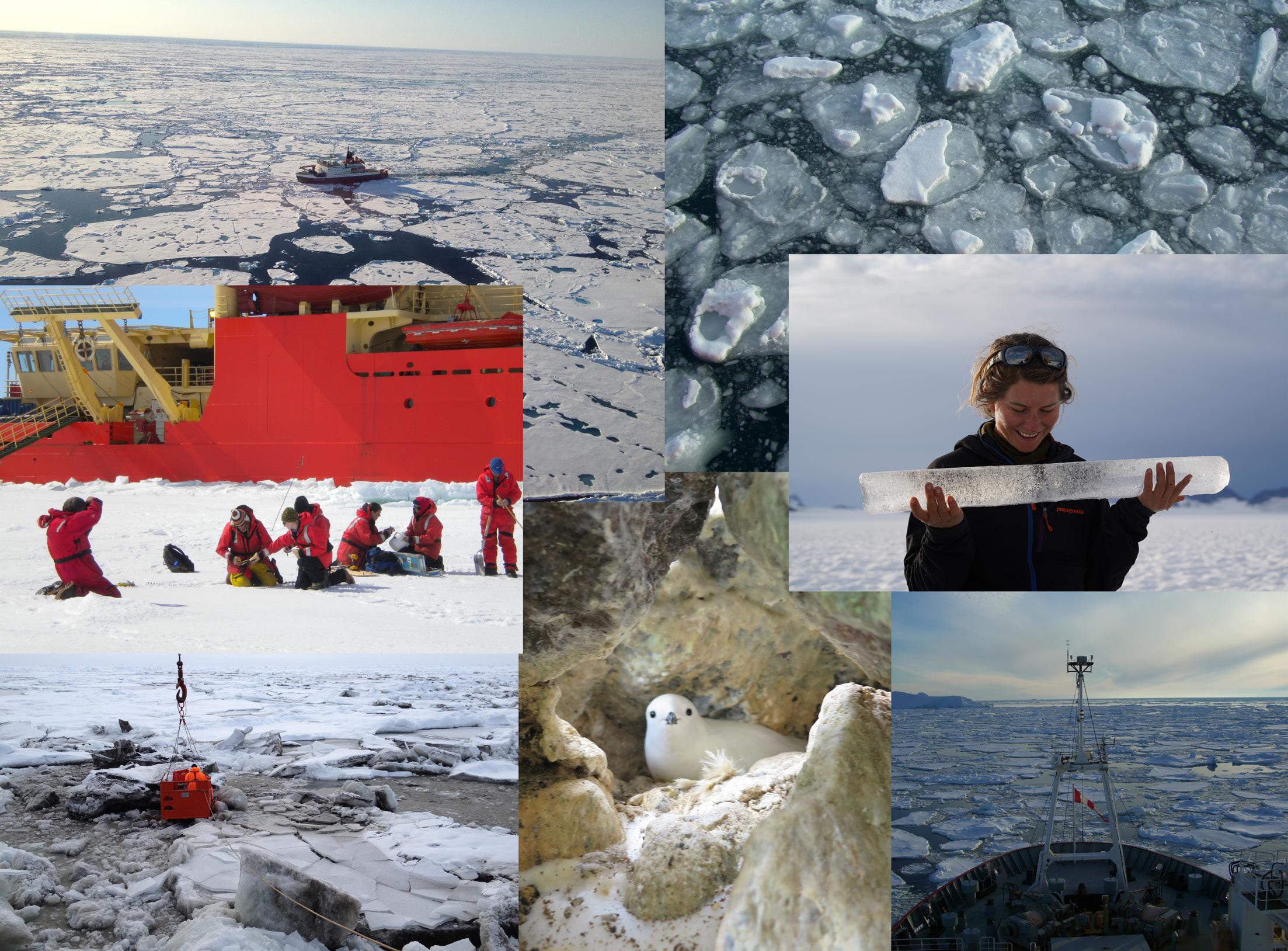
Cover
Collage of images showcasing sea-ice and icecore research at both poles
Photo credits: ruediger Stein, claire Allen, Amy Leventer, bradley Markle and Erin Mcclymont.
PAGES MAGAZINE ∙ VOLUME 30 ∙ NO 2 ∙ OctObEr 2022 CC-BY 66 ANNOUNCEMENTS
About this issue
Sea ice in the polar regions is a very relevant topic today, and the focus of multiple PAGES working groups. two of these groups – Arctic cryosphere change and c oastal Marine
Arctic Cryosphere Change and Coastal Marine Ecosystems t he PAGES working group on Arctic cryosphere change and c oastal Marine Ecosystems (AcME; pastglobalchanges.org/ acme) provides a community platform to critically assess and refine available coastal marine proxies that can be used to recon struct cryosphere changes and their multi faceted ecosystem impacts. AcME seeks to promote a leap forward in the accuracy of paleo reconstructions that are central for de ciphering cryosphere-biosphere interactions in the Arctic region at relevant timescales.
Early-career perspectives on ice-core science
t he Ice c ore Early c areer researchers Workshop (I cEcreW; pastglobalchanges. org/calendar/128625) brought together a diverse group of US-based scientists to discuss past and future ice-core projects, to build community, and to develop 10 articles showcasing the current state and future directions of ice-core science. From millionyear-old samples of the atmosphere to mi crobes living within ice sheets, the I cEcreW early-career participants seek to share with you the immense value of ice cores for un derstanding the Earth system.
For more information and to get involved in ice-core research or to connect with other early-career scientists, go to:

• Ice c ore Young Scientists (I c YS; pastglobalchanges.org/icys)
• Polar Science Early c areer c ommunity Office (PSEccO; psecco.org)
• Association of Polar Early c areer Scientists (APEc S; apecs.is)
• Polar Impact (polarimpactnetwork.org)
Magazine issue. t he following section on ice-core science, by early-career research ers, provides another perspective on research at the poles.
Cycles of Sea-Ice Dynamics in the Earth system

Southern Ocean sea ice plays several impor tant roles within the Earth system, affecting nutrient cycling and marine productivity, as well as modulation of air–sea gas exchange and deep water formation in high latitudes. As sea ice changes in the future, it is impor tant for Earth system models to be able to simulate the effects of these changes.
t he aim of the cycles of Sea-Ice Dynamics in the Earth system (c-SIDE; pastglobalchanges org/c-side) working group is to reconstruct changes in sea-ice extent in the Southern Ocean for the past 130,000 years, recon struct how sea-ice cover responded to global cooling as the Earth entered a glacial cycle, and to better understand how sea-ice cover may have influenced nutrient cycling, ocean productivity, air–sea gas exchange, and circulation dynamics.

PAGES MAGAZINE ∙ VOLUME 30 ∙ NO 2 ∙ OctObEr 2022CC-BY 67ABOUT THIS ISSUE
Ecosystems and cycles of Sea-Ice Dynamics in the Earth system – combined forces to produce the current collection of 12 sci ence highlights in this Past Global Changes
Figure 3: Ice core (Photo credit: NASA's Goddard Space Flight center/Ludovic brucker).
Figure 1: Fresh water and sediment input into the Arctic Ocean are expected to increase with climate change (Photo credit: NASA Earth Observatory/Jesse Allen).
Figure 2: Sea ice in the Southern Ocean (Photo credit: Pearse buchanan).
Meet our guest editors
Matthew Chadwick british Antarctic Survey, c ambridge, UK, and c ornwall Insight, Norwich, UK
Matthew completed his PhD at the british Antarctic Survey in 2021, where he worked on reconstructing Antarctic sea ice during the peak of the last interglacial period. He is now a lead research analyst at c ornwall Insight, researching the latest developments in renewable energy and providing insights to help the UK's energy sector make the transi tion to net zero.


Karen E. Kohfeld

Simon Fraser University, burnaby, bc , c anada
Karen is an Earth systems scientist concentrat ing on understanding climate and the global carbon cycle over glacial–interglacial cycles, using global datasets to test climate models. She also studies regional changes in climate and the carbon cycle, focusing on extreme weather behavior, ocean acidifica tion, carbon storage in coastal wetlands and lacustrine environments, and changes in climate and fire behavior in western c anada
over the last 10,000 years. She is a steering committee member of the PAGES working group cycles of Sea-Ice Dynamics in the Earth System (c-SIDE; pastglobalchanges. org/c-side).
Amy Leventer c olgate University, Hamilton, NY, USA
Amy is a micropaleon tologist, who special izes in paleoclimatic reconstructions of the Antarctic, and modern geologic and biologic processes in the southern ocean. Her teach ing specialties include oceanography, pa leoclimatology, and environmental studies. Amy is the 2018 recipient of the Goldthwait Polar Medal, awarded by the byrd Polar and climate research c enter in recognition of her distinguished record of scholarship and service in polar science.

Anna Pieńkowski
Adam Mickiewicz University, Poznań, Poland, and University c entre in Svalbard, Longyearbyen, Norway
Anna works in the fields of micropale ontology, biogeochemistry, and marine


geology in polar environments. She is a steering committee member of the PAGES working group Arctic cryosphere change and coastal Marine Ecosystems (AcME; pastglobalchanges.org/acme). Her inter ests include studying environmental and climatic response of marine polar regions to global change past and present, the Late Quaternary environmental evolution of Arctic archipelagos, fidelity and appropriate use of biogenic proxies, and marine radiocarbon chronologies. She is currently PI on cHanging Antarctic Marine Environments (cHArME), a project focused on the effects of recent climate warming on Antarctic ecosystems and environments funded by POLS (National Science centre Poland & Norwegian Grants).
Heike Zimmermann Geological Survey of Denmark and Greenland, c openhagen, Denmark
Heike is an expert in paleoecology, working as researcher in the de partment of Glaciology and climate. t here, she studies changes in the cryosphere and marine ecosystems over time using sedimentary ancient DNA. She has participated in several field expeditions to retrieve both ice cores and marine sedi ment cores from polar regions.
PAGES MAGAZINE ∙ VOLUME 30 ∙ NO 2 ∙ OctObEr 2022 68 ABOUT US: SeA ice iN the pol Ar regioNS
Glaciated marine coastal environments are sentinels for climate change (Photo credit: Anna Pieńkowski).
Sea ice in the polar regions
 Matthew chadwick1,2, K.E. Kohfeld3, A. Leventer4, A. Pieńkowski5,6 and H. Zimmermann7
t his special volume highlights advances in sea-ice reconstruction and reflects the efforts of two PAGES working groups: Arctic cryosphere change and c oastal Marine Ecosystems (AcME; pastglobalchanges.org/ acme) and cycles of Sea-Ice Dynamics in the Earth System (c-SIDE; pastglobalchanges. org/c-side). t his joint effort recognizes the large-scale and rapid changes happening in the high latitude oceans, where changes in sea-ice extent are central to a wide range of cascading and interconnected impacts. both working groups address paleo sea-ice recon struction as a tool for understanding broad ecosystem changes that have occurred in the past. t his research provides a longer-term perspective on modern changes, and these data can be used to constrain models used to understand today's evolving cryosphere. Our articles are dedicated to overviewing the proxies we have to reconstruct past seaice conditions, their different use between the Northern and Southern hemispheres, and across different timescales.
t his volume starts with articles highlight ing recent changes in sea-ice distribution and extent in the Arctic and Antarctic with satellite-based data by Meier (p. 70), il lustrating the differences in change at the two poles. Wilson et al. (p. 72) focus on a Sikumiut community-based sea-ice monitor ing program that highlights the important contributions of historical knowledge from an Inuit community directly facing changes that impact safe travel over the sea ice. Fogt et al. (p. 74) compare satellite-based data with ice-core-based paleo reconstructions from the past century to address regional differences in Antarctic sea-ice extent, and
investigate the teleconnections and forcings responsible for spatial variability in recent trends. tedesco and Post (p. 76) describe polar marine ecosystems associated with sea ice; understanding these modern systems is fundamental to the application of proxies to reconstruct past sea ice.
reconstructing sea ice further back in time requires advances in novel proxies and more traditional and established prox ies. Armbrecht (p. 78) and Harðardóttir (p. 80) present the state of knowledge in using ancient DNA in Antarctic and Arctic marine sediments, respectively, to track taxa through time; this promising and versa tile toolkit offers new ways to identify and quantify sea-ice species, and to reconstruct ecosystems in regions where most taxa do not have hard parts preserved. Similarly, Mc clymont et al. (p. 82) propose the use of snow petrel stomach-oil deposits as a new proxy for sea ice in Antarctica, based on their foraging habits; the authors' data, extending to the last glacial period, indicates the role that coastal polynyas may have played as refugia during a time of expanded sea-ice extent. Finally, Nixon (p. 84) reviews the use of geomorphic characteristics of raised beaches, and the cautious interpre tation of the presence of whale bones and driftwood to develop low-resolution records of paleo sea-ice extent, which can augment the higher resolution records derived from marine sediment cores.
Glacial–interglacial patterns of sea-ice variability in both the Antarctic (chadwick p. 86; Jones et al. p. 88) and Arctic (Stein et al. p. 90; Sicard et al. p. 92) focus on the
"warmer-than-modern" period of Marine Isotope Stage 5e as a potential analog for environmental conditions that we might an ticipate by the end of the century as global average temperatures continue to rise. reconstructions are based on a combination of proxies, including microfossils (diatoms) and biomarkers; these proxy data provide important ground-truthing for scientists to compare with models that simulate sea-ice extent. c ombining the two – paleoreconstructions and modeling – provides a path forward for understanding the likely changes in sea-ice distributions in the near future. Finally, de Vernal and Hillaire-Marcel (p. 94) look back much further in time, to the Quaternary (the last 2.58 million years); they highlight the timing of the develop ment of seasonal sea ice, with most of the Quaternary characterized by perennial seaice cover that limited light penetration and primary production.
t he papers in this volume highlight recent advances in paleo sea-ice reconstruction; however, challenges remain for future re search, including:
(1) c ontinued development of our use and understanding of novel proxies that allow us to investigate the vast parts of polar oceans where shells and tests are not preserved;
(2) critically questioning our use and un derstanding of traditional proxies to refine them;
(3) Linking the observed sea-ice changes to associated changes in nutrients, marine ecosystems, ocean circulation, and carbon cycling;
(4) Accounting for traditional knowledge in sea-ice reconstructions;
(5) Using these new developments to improve our modeling of these sea-ice feed backs; and


(6) Understanding the relative timing of changes between the two polar regions.
AFFILIAtIONS
1british Antarctic Survey, c ambridge, UK
2c ornwall Insight, Norwich, UK
3School of resource and Environmental Management and School of Environmental Science, Simon Fraser University, burnaby, bc , c anada
4Department of Geology, c olgate University, Hamilton, NY, USA
5Institute of Geology, Adam Mickiewicz University, Poznań, Poland
6Department of Arctic Geology, University c entre in Svalbard (UNIS), Longyearbyen, Norway
7Geological Survey of Denmark and Greenland, c openhagen, Denmark
cONtAct
Amy Leventer: aleventer@colgate.edu
PAGES MAGAZINE ∙ VOLUME 30 ∙ NO 2 ∙ OctObEr 2022 CC-BY 69EDITORIAL: SeA ice iN the pol Ar regioNS
doi.org/10.22498/pages.30 2.69
Figure 1: Efforts to reconstruct paleo sea-ice distribution use a variety of proxies, including diatoms, pictured here, as well as biogeochemical markers, that are recovered from sediment and ice cores. Photo credits: Madeline roy (top left), bradley Markle (bottom right), Amy Leventer (top right and bottom left).
Sea ice in the satellite era
Walter N. Meier
Sea ice during the modern satellite observational record shows a stark contrast between the Arctic and Antarctic. The Arctic is undergoing profound change with significant declines in extent and thickness. The Antarctic is marked by strong variability and small trends.
Indigenous populations have been exploring the Arctic environment since they arrived in the region thousands of years ago. recorded observations of sea ice date to the time of the first European exploration of the polar regions, taken from on the ice or from ships, as early as the 1600s. Antarctic observations are more recent, with little data before the early 1900s. t he advent of aircraft brought the ability to do aerial reconnaissance, and this, along with ship observations, provided the basis for early sea-ice charts that date back to the 1920s in some regions (Walsh et al. 2017). beginning in the mid-1960s, early satellite data from visible and infrared sensors provided the first views of sea ice from space (Meier et al. 2013). Other satel lite sensors provided intermittent coverage through the mid-1970s. However, the mod ern satellite record began with the advent of multi-frequency passive microwave sensors, beginning with the launch of the Scanning Multichannel Microwave radiometer (SMM r) on the NASA Nimbus-7 platform in October 1978. SMM r was succeeded by a
series of similar instruments on U.S. Defense Department platforms that continue to oper ate today.
Passive microwave sensors are particu larly useful for polar sea ice (Steffen et al. 1992). First, they sense the Earth's emitted microwave radiation, and thus, unlike visible sensors, they do not rely on solar illumina tion. Second, the frequencies employed are generally transparent to clouds. t his allows for retrieval of sea-ice information in all sky conditions, including through clouds and in darkness. t he sensors view the polar regions at least once per day, except for a region surrounding the pole (the size of which has varied over time). t his has provided a nearcomplete and continuous record of sea-ice concentration and extent for over 40 years. t here are some limitations to passive micro wave records of sea ice. t he spatial resolu tion is relatively low over much of the record, on the order of 25 km. Also, retrievals can be biased in some conditions, particularly summer melt, thin/new ice, and near the ice
edge. Nonetheless, the data are robust for hemispheric or regional assessments of the sea-ice cover (e.g. Parkinson and DiGirolamo 2021; c omiso et al. 2017).
Sea-ice concentration and extent trends t he most common climate indicators from sea ice are concentration and extent. c oncentration is the fraction coverage (usually in percent) of ice in a given region. Extent is the total area that is covered by ice above a given concentration threshold (often 15%, as is used here); using a threshold ame liorates the effect of the concentration bias due to melt and thin ice.
Here we use estimates from the NSID c Sea Ice Index (Fetterer et al. 2017), based on the NASA team algorithm (c avalieri et al. 1984), to examine changes in the sea-ice cover during the passive microwave satellite record. First, we present trends in monthly average extent over the full 43-year record January 1979 through December 2021. We use a standardized anomaly approach,
PAGES MAGAZINE ∙ VOLUME 30 ∙ NO 2 ∙ OctObEr 2022 CC-BY 70 SCIENCE HIGHLIGHTS: SeA ice iN the pol Ar regioNS
doi.org/10.22498/pages.30 2.70
Figure 1: Monthly standardized sea-ice extent anomalies (thin solid lines) for the Arctic (blue) and Antarctic (red) for January 1979 through December 2021 (x-axis) with 12-month running averages (thick solid lines) and trend (dashed lines). Data from the NSIDc Sea Ice Index (Fetterer et al. 2017).
-5 -4 -3 -2 -1 0 1 2 3 4 5 1979 1985 1991 1997 2003 2009 2015 2021 Standardized Anomal y Arctic Antarctic
(Fetterer et al.
where the monthly anomalies (relative to the 1981 to 2010 climatology) are normalized by the standard deviation for each month (over the climatology period). t his approach accounts for the large seasonal variation in extent through the year. t he extent trends (Fig. 1) illustrate the difference between the Arctic and Antarctic sea-ice evolution over the satellite record. While there is interan nual variability in the Arctic sea-ice extent, there is a clear downward trend. In contrast, the Antarctic has a small upward trend in extent, but with high interannual variabil ity. Particularly notable in the Antarctic is a sharp drop between 2015 and 2017, where the anomaly went from a record high in the satellite record to a record low; this has been associated with changes in atmospheric circulation (Wang et al. 2019).
t he contrast is also evident in extent trends for individual months. For example, the Arctic extent trend (±2 standard deviations) is -39,800 ± 6,300 km2 /yr for March and -81,100 ± 13,000 km2 /yr for September. both of these months, and indeed all months, are statistically significant at the p < 0.05 level. In contrast, the Antarctic extent trend is +7,900 ± 13,300 km2 /yr for March and +8,700 ± 10,100 km2 /yr for September. t he monthly trends for the Antarctic are either not significant at the p < 0.05 level or only marginally significant.
t he spatial distribution of the changes in the sea-ice cover are also distinctly different between the north and the south, as seen in concentration trends (Fig. 2). t he Arctic shows decreasing concentration in virtually all regions where there is interannual vari ability. In the Antarctic, some regions show an increase in concentration, while others show a decrease, consistent with the nearzero overall extent trends.
Sea-ice age and thickness

Sea-ice extent and concentration data provide information about the surface of the ice, but these are only a partial indication of changes in the ice cover. What is missing is the third dimension: thickness and volume. Unfortunately, long-term data on thickness and volume are limited, with only intermit tent and sparse thickness measurements from submarine sonars or drill holes at field camps. t he longest complete records, starting in the early 1980s, rely on proxy estimates using ice type or ice age and are typically only available for the Arctic. Older ice is generally thicker ice, so changes in the age of the ice indicate changes in thickness. One such age product indicates a nearly complete loss of Arctic ice older than four years ( tschudi et al. 2020). Such ice once comprised over 30% of the Arctic Ocean in the mid-1980s, but now covers less than 5% of the region.


More recently, satellite altimeters have facili tated direct estimates of thickness (e.g. Petty et al. 2020; Laxon et al. 2013). t he algorithms to derive thickness from the surface eleva tion data are still not completely mature, and there are potentially large uncertainties, particularly due to lack of information on the overlying snow cover. However, the data can now provide reasonable estimates of inter annual variability and trends in Arctic thick ness and volume. Since 2003, a substantial thinning of the ice cover has been observed (e.g. Kacimi and Kwok 2022), which is con sistent with the loss of the older ice types. Augmenting the satellite data with earlier submarine data shows a long-term loss of thickness since the 1970s (Kwok 2018).
Unfortunately, due to the nature of Antarctic sea ice (thinner ice, thicker snow cover, substantial melt), altimetry data are not reli able, and tracking of age is less effective. So, there is little information on sea-ice age or thickness trends. However, because much of the Antarctic sea-ice cover is seasonal (i.e. melts completely each summer) and the trends in extent and concentration are small, changes in thickness and volume are likely similarly small.


Summary
Over the period of the continuous satel lite record, Antarctic sea ice is marked by regional and interannual variability, with minimal trends in the ice cover. In contrast, Arctic sea-ice extent and concentration are significantly decreasing throughout the re gion; the ice is thinning, and older ice types are disappearing. In short, Arctic sea ice is an environment in transformation. It is under going changes far beyond natural variability in response to increases in temperature. If such warming trends continue, it is likely that the Arctic Ocean will become largely season ally ice-free in the coming decades.
AFFILIAtION
National Snow and Ice Data c enter, c ooperative Institute for research in Environmental Sciences, University of c olorado, boulder, USA
cONtAct
Walter N. Meier: walt@colorado.edu
rEFErENcES
cavalieri DJ et al. (1984) J Geophys res 89: 5355-5369 comiso Jc et al. (2017) J Geophys res 122: 6883-6900
Fetterer F et al. (2017) Sea Ice Index, Version 3, National Snow and Ice Data center, Accessed 14 July 2022 Kacimi S, Kwok r (2022) Geophys res Lett 49: e2021GL097448
Kwok r (2018) Env res Lett 13: 105005
Laxon SW et al. (2013) Geophys res Lett 40: 732-737
Meier WN et al. (2013) cryosphere 7: 699-705

Parkinson cL, DiGirolamo NE (2021) rem Sens Environ 267: 112753
Petty AA et al. (2020) J Geophys res 125: e2019Jc015764
Steffen K et al. (1992) In: carsey F (Ed) Microwave remote sensing of sea ice. American Geophysical Union, Geophysical Monograph 68: 201-231
tschudi MA et al. (2020) cryosphere 14: 1519-1536
Walsh JE et al. (2017) Geogr rev 107: 89-107
Wang Z et al. (2019) J climate 32: 5381-5395
PAGES MAGAZINE ∙ VOLUME 30 ∙ NO 2 ∙ OctObEr 2022CC-BY 71SCIENCE HIGHLIGHTS: SeA ice iN the pol Ar regioNS
Figure 2: concentration trends (% per decade) for the Arctic and Antarctic for March and September. Only trends at the p < 0.05 significance level are shown. Adapted from the NSIDc Sea Ice Index
2017). Arctic Mar Arctic Sep Antarctic Mar Antarctic Sep
An inuit sea-ice-change atlas from Mittimatalik, Nunavut
For the first time, Inuit have used their sea-ice knowledge to reconstruct historical sea-ice conditions to address climate change and resource development implications for safe sea-ice travel in their region.
t he Inuit community of Mittimatalik (Pond Inlet) is located in the c anadian High Arctic (Fig. 1). traveling on the sea ice is central to the wellbeing, identity, and culture of the Mittimatalingmiut (residents of Mittimatalik). t he nearby floe edge is a highly anticipated sea-ice feature that is present from late December to early July (Fig. 1). It provides a stable, landfast, sea-ice platform to hunt and fish near the open water. Although Inuit have always experienced and adapted to variable ice conditions, changes in ice conditions are now beyond what they would consider normal (Pearce et al. 2010). t herefore, Inuit are looking for additional information to support their safe travel decision-making. However, there is a gap in the availability of current sea-ice climate products. For example, outputs from sea-ice models are not at community scale, and sea-ice charts from national ice services capture the openwater summer shipping season, and not
to July in Mittimatalik) (Wilson et al. 2021).
With a variety of near real-time and archived satellite imagery now publicly available, Inuit training, to interpret satellite imagery and create their own maps, is the missing step to support community-based sea-ice mapping (Laidler et al. 2011; Segal et al. 2020).

Mittimatalingmiut are already dealing with the impacts of climate change on sea-ice conditions, compounded by the pressure to increase commercial shipping in early July through the sea ice to the nearby Mary river iron-ore mine and port (Fig. 1). A local committee of Inuit sea-ice experts, called Sikumiut, identified the need to document the region's historical sea-ice conditions to understand: (1) where the sea ice was becoming more dangerous, to adapt their travel routes; and (2) the potential impacts of shipping earlier to the mine. Here we de scribe the process of co-creating a 23-year
with Sikumiut, how the satellite imagery and geographic information system (GIS) map ping tools and training were put in the hands of Inuit with knowledge and experience of traveling on the ice, and how the atlas differs from other products to help address Inuit priorities.
What is Sea Ice Inuit Qaujimajatuqangit ?
Inuit maintain the longest unrecorded climate history of sea ice in c anada.
Mittimatalik's sea-ice climatology is pre served by orally passing down this knowl edge and sharing their extensive and recent travel experiences on the sea ice (called Inuit Qaujimajatuqangit, or IQ). Sikumiut's deep climatological knowledge of the seasonal evolution of sea ice is what keeps them safe while traveling on it. However, their sea-ice IQ is not in a database, but exists in the col lective minds of these expert sea-ice travel ers. Also, their climatology is not focused on
PAGES MAGAZINE ∙ VOLUME 30 ∙ NO 2 ∙ OctObEr 2022 CC-BY 72 SCIENCE HIGHLIGHTS: SeA ice iN the pol Ar regioNS
Katherine
Wilson1,2, A. Arreak1,3, Sikumiut committee3 and t bell1,2 doi.org/10.22498/pages.30 2.72 Figure 1:
Map of the Mittimatalik sea ice travel region, Nunavut, canada. background satellite image: MODIS true color composite, 9 June 2019 (NASA 2019).
Ar regioNS
a general scientific sense, but more specifi cally on ice conditions for safe travel.
Making an IQ-based sea-ice change atlas
In 2019, a pilot curriculum was developed to train Andrew Arreak, an Inuit community researcher from Mittimatalik, in satellite imagery interpretation and GIS. In 2020, Arreak interpreted over 2000 radarsat ScanSar Wide (1997 to 2019) and MODIS (2000 to 2019) images over six weeks (18 June to 29 July) to capture the evolution of spring ice-travel conditions prior to breakup.
Arreak created weekly maps to digitize areas of sea ice that were no longer safe for travel, as the warmer temperatures began to melt the snow and sea ice. Arreak's sea-ice travel knowledge, and that shared with him by Sikumiut members, allowed him to moni tor known areas in the satellite imagery for rapid change due to river outflow, melting glaciers, strong ocean currents, and recur ring leads (cracks that stay open in the ice).
Digitized maps were converted to raster to create maps to: (1) depict average ice travel conditions for each week of breakup based on the 23-year record, and (2) capture the spatial evolution of breakup for each year. Arreak was also trained in statistical analysis to review spatial and temporal trends in the sea-ice-breakup maps.
What the atlas tells us about sea-ice breakup
Snowmelt on the land signals the start of the breakup season. t he average onset of snowmelt in the 23-year record was detect able in the satellite imagery the week of 11–17 June. by the following week of 18–24 June, areas of open water became visible in the satellite imagery in the southeast inlets and mouths of local rivers (Fig. 2). It is normal for the floe edge to fracture and break off to form new edges during the breakup season. Areas of breakup expand in the south and southeast sounds and inlets, and along the coastlines, until travel to the floe edge is no longer safe by the week of 9–15 July. t he floe edge normally breaks up the week of 16–22 July. However, there was high variability in the timing of sea-ice breakup, and only the week of 2–8 July showed a trend towards earlier breakup with an R 2 value of 0.34 ( p value < 0.5).
Sikumiut has discussed that the floe edge is not as stable as it has been in the past. In reviewing the satellite imagery, the normal breakup date for the floe edge was 18 July (±2 days) between 1997 and 2019. Our results show a trend towards earlier breakup (R 2 = 0.42, p < 0.05) with 7 July 2019 being the earliest breakup date in the record.
Implications for safe ice travel
In 17 out of 23 years (74%), the floe edge fractured to a location called Ukkuanguaq (Figs. 1, 2). Additionally, in 16 out of these 17 years, Ukkuanguaq is the last floe-edge loca tion before the sea ice completely breaks up. Sikumiut already knew of the significance of the Ukkuanguaq; however, this mapped evidence supports community sea-ice adap tation needs. For example, talks are already underway to position time-lapse cameras
shows the spatial pattern for an unusually early breakup. (B) the 2005 map illustrates the spatial pattern for an unusually late breakup. (C) the 2006 map provides an example of a year when the sea ice at the floe edge breaks last.
and other monitoring equipment at this loca tion to provide Mittimatalingmiut advance notice of breakup (bell et al. 2020).
t he average patterns for where and when the sea ice becomes dangerous for travel and the evolution of breakup were consis tent with Sikumiut's IQ. However, Arreak explained that in some years the sea ice in front of the community can breakup earlier than at the floe edge (Fig. 2c). to continue to hunt and fish, Mittimatalingmiut will travel overland to access the sea ice just past Ukkuanguaq. t he GIS-derived summary breakup maps did not capture this pattern, so we reviewed the individual yearly maps. t his type of breakup pattern occurred about half of the time (48%), and there was no apparent increase in the frequency of this pattern over the last decade. Nevertheless, given the importance of hunting at the floe edge, there have been discussions within the community to build a road to Ukkuanguaq as an adaptation strategy to maintain their hunting and fishing activities at the floe edge.
t he IQ-based sea-ice atlas also shows that extending the shipping season into the first two weeks of July could accelerate the breakup of the floe edge, shortening the sea-ice travel season further. If shipping is extended into the breakup season to sup port mining activities, Mittimatalingmiut now have a baseline of their local sea-ice condi tions with which to compare and provide evidence for any future cumulative effects.
Conclusion
Siku asijjipallianinga differs from typical sea-ice climate atlases in that it used western

tools to capture the collective IQ climato logical sea-ice history of the region. Without Sikumiut's and Arreak's IQ and guidance, we would not have been able to interpret the satellite imagery or analyze its results from such an on-ice travel perspective. because this atlas was created from an Inuit viewpoint, it provides an adaptation tool that Mittimatalingmiut can use to share locations of known and changing sea-ice conditions to plan for safe sea-ice travel. t he atlas also clearly demonstrates the scientific merit of IQ in environmental assessments that can potentially impact the future sea-ice regime.
AFFILIAtIONS
1SmartI cE Sea Ice Monitoring & Information Services Inc., St. John's, NL, c anada
2Department of Geography, Memorial University of Newfoundland, St. John's, NL, c anada
3Sikumiut Management c ommittee, Mittimatalik, Nunavut, c anada
cONtAct
Katherine Wilson: katherine@smartice.org
rEFErENcES
bell t et al. (2020) Sikumiut perspectives on monitor ing ice breakup near Mittimatalik: Summary workshops report. St. John's: Unpubl. Available at SmartIcE Inc. with permission
Laidler GJ et al. (2011) can Geogr 55: 91-107
NASA (2019) EOSDIS Worldview: worldview.earthdata. nasa.gov
Pearce t et al. (2010) Polar rec 46: 157-177
Segal r A et al. (2020) Arctic 73: 461-484
Wilson K et al. (2021) Front clim 3: 715105
PAGES MAGAZINE ∙ VOLUME 30 ∙ NO 2 ∙ OctObEr 2022CC-BY 73SCIENCE HIGHLIGHTS: SeA ice iN the pol
Understanding differences in Antarctic sea-iceextent reconstructions in the ross, Amundsen, and Bellingshausen seas since 1900 ryan L. Fogt1, Q. Dalaiden2,3 and M.S. Zarembka1
Antarctic sea-ice-extent reconstructions provide needed historical context to the large variability depicted in the short satellite observations. However, it is important to be mindful of their uncertainties, especially when comparing reconstructions based on paleoclimatological and instrumental data.
t he South Pacific sector of the Antarctic coastline, consisting of the (moving east from the dateline) ross, Amundsen, and bellingshausen seas, has demonstrated some of the strongest trends in Antarctic sea-ice extent since the satellite era (1979; Parkinson 2019). t he annual mean seaice concentration trends (expressed as % per decade) from 1979–2020 (Fig. 1a) show statistically significant increases in the western ross Sea and decreases in the bellingshausen Sea near the Antarctic Peninsula. Even with significant trends, these regions are marked with strong interan nual sea-ice variability partly influenced by teleconnections from the tropics (Holland and Kwok 2012; Meehl et al. 2016; Purich et al. 2016).
to help place the trends depicted by the short time period of satellite observations in a longer historical context, several seaice reconstructions for the South Pacific sector based on both paleoclimatological records and instrumental observations have been created. Abram et al. (2010) used the chemical information from an ice core from the Antarctic Peninsula to reconstruct the annual sea-ice edge in the bellingshausen Sea (70°W–110°W) in the years 1900–2004. Similarly, a later study by t homas and Abram (2016) reconstructed the annual mean seaice edge at 146°W for the years 1702–2010, marked as a green dot in Figure 1a.
to understand processes behind the seaice-extent changes on longer timescales, Dalaiden et al. (2021) combined ice-core and tree-ring-width records with an Earth system model through a data assimilation method to provide annual historical estimates of not only sea-ice extent and concentration, but also the atmospheric circulation (tem perature, pressure, winds) during the years 1800–2000. More recently, Fogt et al. (2022) reconstructed seasonal sea-ice extent in the sectors from raphael and Hobbs (2014) from 1905–2020 using a principal component regression technique that employed obser vations of pressure and temperature across the Southern Hemisphere, and indices from leading modes of climate variability known to influence Antarctic sea-ice extent. Despite the potential to increase the understanding of historical sea-ice variations from these re constructions, Fogt et al. (2022) noted a very weak interannual correlation between these
datasets, making it challenging to know the reliability and usefulness of each dataset; yet understanding these uncertainties and dif ferences is fundamental to ensure a correct application of the reconstructions.
South Pacific Antarctic sea-ice extent since 1900
Figure 1b shows the annual mean (ap proximately related to the August–October values for the Abram et al. (2010) recon struction) sea-ice reconstructions for the Amundsen– bellingshausen seas (top panel) and ross–Amundsen seas, along with satel lite observations. Importantly, the Fogt et al. (2022) reconstruction was explicitly calibrated to the satellite observations, so it is not surprising that it agrees the best with the observed values in both regions. In contrast, the Dalaiden et al. (2021) recon structions are not calibrated to observations, but rather are extracted (here, using the raphael and Hobbs (2014) sectors) from the climate model simulation that is guided by paleoclimatological data. t hese differences in methodology certainly contribute to
a)Annual Mean Sea Ice Concentration Trend, 1979 2020
the differences among the various recon structions, since there is more agreement between the paleo-based reconstructions (all except Fogt et al. 2022) than between the paleo-based and instrument-based (only Fogt et al. 2022) reconstructions.
Nonetheless, the recent changes are cap tured to varying degrees by all the recon structions, showing decreases after 1979 in the Amundsen– bellingshausen seas, and increases in the ross-Amundsen seas (Fig. 1b). Prior to 1979, however, there are notable differences in the average sea-ice condi tions, with opposite behavior between the paleo-based and Fogt et al. (2022) recon structions. In the Amundsen– bellingshausen seas, the paleo-based reconstructions frequently indicate above average sea-ice extent in the early-to-mid 20th century, whereas the Fogt et al. (2022) reconstruc tion indicates below average sea-ice extent during this time (Fig. 1b, top). t he variability is opposite in the ross-Amundsen seas: here the paleo-based reconstructions frequently indicate below average sea-ice extent in the
b)Sector Annual Mean Sea Ice Extent 1900 2020
Figure 1: (A) Sea-ice concentration trends (% per decade) from 1979-2020, with areas of stippling indicating trends that are statistically different from zero at p < 0.05. the lines denote the sectors used to define the sea-ice extent – with the dashed lines showing the sectors established by Parkinson (2019) and the solid lines sectors defined by raphael and Hobbs (2014). (B) timeseries of annual mean (August–October for Abram et al. 2010) standardized sea-ice extent for the Amundsen–bellingshausen seas (top row) and ross–Amundsen seas (bottom row).
PAGES MAGAZINE ∙ VOLUME 30 ∙ NO 2 ∙ OctObEr 2022 CC-BY 74 SCIENCE HIGHLIGHTS: SeA ice iN the pol Ar regioNS
doi.org/10.22498/pages.30 2.74
Sea Level Pressure Trends
Figure 2: (A) thirty-year running trends of the standardized sea-ice-extent timeseries from Figure 1b. the magnitude of the trend (in standard deviations per decade) is shaded, and stippling indicates 30-year trends that are statistically different from zero at p < 0.05. (B) Annual mean sea-level pressure trends (shaded, in hPa per decade) for 1905–1979 (left column), 1979–end (middle column), and the full time period (right column). the top row is the sea-level pressure from the Dalaiden et al. (2021) simulation (which ends in 2000), and the bottom row is the merged seasonal pressure dataset (annually averaged) from Fogt and connolly (2021), which ends in 2013. Stippling indicates trends that are statistically different from zero at p < 0.05.

early-to-mid 20th century, while the Fogt et al. (2022) reconstruction indicates above av erage sea-ice extent prior to the onset of sat ellite observations (Fig. 1b, bottom). Perhaps surprisingly, the correlations with observed sea-ice concentration are all fairly similar spatially (not shown), which suggests that the various regions represented by each recon struction is a smaller contributing factor to the disagreement in the reconstructions.
to highlight the differences further, 30year running trends of the annual mean reconstructions are provided in Figure 2a. Notably, the paleo-based reconstructions all suggest that the sign (and often statistical significance) of the observed trends for the two regions continue throughout the 20th century. In contrast, the Fogt et al. (2022) trends indicate a change in the sign (and often statistical significance) of the trends prior to 1979.
The role of atmospheric circulation
Since Dalaiden et al. (2021) reconstructed the historical changes of the atmosphere, it is possible to also investigate changes in the atmospheric circulation in relation to sea-ice trends. Additionally, Fogt and c onnolly (2021) provide another pressure dataset, which employs a seasonal, spatially com plete reconstruction poleward of 60°S (Fogt et al. 2019) and the National Oceanic and Atmospheric Administration 20th-century reanalysis (Slivinski et al. 2019) equatorward of 60°S. Importantly, the Fogt and c onnolly (2021) merged pressure dataset avoids large artificial trends in other datasets over Antarctica prior to 1957 and, therefore, likely provides a more robust estimate of 20thcentury pressure trends (Fogt and c onnolly 2021). Annual sea-level pressure trends from the two datasets are displayed in Figure 2b. In agreement with the sea-ice trends, the pressure trends from Dalaiden et al. (2021) are the same throughout the 20th century,
although not statistically significant prior to 1979. In contrast, but consistent with the instrument-based sea-ice reconstructions of Fogt et al. (2022), the pressure trends in the merged pressure dataset from Fogt and c onnolly (2021) show a reversal in pressure trends across Antarctica before and after 1979. Since a large portion of the Antarctic sea-ice extent in this region is driven by the atmospheric circulation, Figure 2b demon strates that changes in the atmospheric cir culation give rise to the differences between the Fogt et al. (2022) reconstructions and those derived from paleoclimatological data.
Discussion
Further work is planned to better under stand the origin of these differences, with particular attention paid to the atmospheric circulation reconstruction. In contrast with the paleo-based reconstruction, the instrument-based reconstruction strongly relies on large-scale climate patterns depicted in the observations, but may not fully represent the regional and highly vari able Antarctic weather that may be better captured by ice cores closer to the Antarctic sea-ice edge. t herefore, the impact of the geographical locations of the observations used in the reconstructions will be analyzed through several sensitivity experiments by including additional records, such as the near-surface air temperature and surfacepressure records from Antarctic weather stations – available since 1958 – and coral records situated in the tropical Pacific. t hese sensitivity experiments will aid in unlock ing the contribution to regional Antarctic sea-ice variations from large-scale telecon nections, including tropical teleconnections, which have been demonstrated to play a substantial role in the Antarctic climate over the instrumental period (Holland and Kwok 2012; Meehl et al. 2016; Purich et al. 2016) on much longer timescales.
AFFILIAtIONS
1Department of Geography and Scalia Laboratory for Atmospheric Analysis, Ohio University, Athens, USA
2Université catholique de Louvain (U cLouvain), Earth and Life Institute (ELI), Louvain-la-Neuve, belgium
3Fonds de la recherche Scientifique FrS-FN rS, brussels, belgium
cONtAct r yan Fogt: fogtr@ohio.edu
rEFErENcES
Abram NJ et al. (2010) J Geophys res 115: D23101
Dalaiden Q et al. (2021) clim Dyn 57: 3479-3503
Fogt rL, connolly c J (2021) J clim 34: 5795-5811
Fogt rL et al. (2019) clim Dyn 53: 1435-1452
Fogt rL et al. (2022) Nat clim chang 12: 54-62
Holland Pr, Kwok r (2012) Nat Geosci 5: 872-875
Meehl GA et al. (2016) Nat Geosci 9: 590-595
Parkinson cL (2019) Proc Natl Acad Sci USA 116: 14,414-14,423
Purich A et al. (2016) J clim 29: 8931-8948
raphael MN, Hobbs W (2014) Geophys res Lett 41: 5037-5045
Slivinski Lc et al. (2019) Q J r Meteorol Soc 145: 2876-2908
thomas Er, Abram NJ (2016) Geophys res Lett 43: 5309-5317
PAGES MAGAZINE ∙ VOLUME 30 ∙ NO 2 ∙ OctObEr 2022CC-BY 75SCIENCE HIGHLIGHTS: SeA ice iN the pol Ar regioNS
a) Annual Mean Sea Ice Extent, 30 year Running Trends b) Annual Mean
Sea ice: An extraordinary and unique, yet fragile, biome
Letizia tedesco1 and Eric Post2
Sea ice – a unique and extraordinary biome in its nature and dynamics – is under threat. Ocean warming, sea-ice decline, and altered seasonality endanger the simple, vulnerable, and low resilient sea-ice and ice-associated food webs in both polar oceans.
Sea ice is one of the largest biomes on our planet, covering an area up to 14 million km2 in the Arctic Ocean in March 2022 and up to 17 million km2 in the Southern Ocean last September. While Arctic and Antarctic sea ice are similar in many facets, fundamental differences also affect the type of sea-ice biome they are associated with. t he fact that the Arctic Ocean is surrounded by land makes the sea ice there more stationary, per manent, and deformed, and with more melt ponds due to a thinner snowpack (Fig. 1a). In contrast, the Southern Ocean surrounds an entire continent. It is affected by abundant precipitation with more snow-ice formation, more mobile sea ice prone to openings, and more young ice formation (Fig. 2a).
Since satellite records began providing reli able observations over 40 years ago, Arctic sea ice has steadily decreased annually in every season, reaching an annual minimum extent in summer, and first-year ice has replaced multiyear ice as the dominant ice type (Stroeve and Notz 2018). During the same period, Antarctic sea ice has shown strong regional and seasonal patterns of variability, with gradual increases in extent until a reversal of this trend in 2016. Since then, it has declined at a rate far exceeding that of Arctic sea ice (Parkinson 2019). Under a warming scenario of at least 2.0° c , the Arctic Ocean is expected to become ice-free throughout September regularly (Notz and Stroeve 2018). Sea ice in the Southern Ocean is also projected to decrease significantly in all seasons during this century in response to warming, with a larger spread of uncertainty in model estimates (Holmes et al. 2022).
The sea ice and ice-associated food webs Sea ice is an extraordinary multiphase medium comprising a solid ice matrix, liquid salty brines, gas bubbles, and impurities. It is in the brines that a unique ecosystem
develops. From viruses, fungi, bacteria, and microalgae to different forms of meio- and macrofauna, an entire food web inhabits sea ice (Figs. 1b, 2b). c ompared to the Arctic, Antarctic sea ice is typically more snowcovered, insulated, and permeable, and contains more extensive brines, facilitating access by larger organisms. t he most abun dant group of organisms found in sea ice is usually tiny algae, which, together with their pelagic counterpart, phytoplankton, form the base of the entire polar marine food web.
In both hemispheres, and in both land-fast and pack ice alike, different algal species, often representing a single functional group, dominate; these include autotrophic flagel lates in surface layers, mixed communities in the interior layers, and pennate diatoms in bottom layers (van Leeuwe et al. 2018; Figs. 1b, 2b). Among pennate diatoms, those of the genus Nitzschia are often dominant in both Arctic and Antarctic sea ice. rotifers and nematodes are more commonly found in Arctic sea ice, while copepods are more commonly found in Antarctic sea ice (bluhm et al. 2017; Figs. 1b, 2b). crustaceans domi nate under-ice communities. c opepods and amphipods are found in both under-ice en vironments; dominant taxa include euphau siids in the Southern Ocean and amphipods in the Arctic Ocean (Figs. 1b, 2b). Ice algae support key under-ice foraging species, i.e. Arctic cod (Boreogadus saida) in the Arctic Ocean (Fig. 1a, c) and Antarctic krill (Euphausia superba) in the Southern Ocean (Fig. 2). t hese species are dependent on the existence of stable sea ice and are key for transferring carbon from primary producers to higher trophic levels, from fish to marine mammals to humans (Figs. 1, 2).

Sea ice and terrestrial ecology
Strong linkages exist between Arctic marine and terrestrial ecology (Fig. 1c). Sea ice
can act as an important ecological cor ridor, connecting land masses in the Arctic and thereby facilitating the exchange of individuals of some terrestrial species among populations. Moreover, sea ice is an important foraging and predator-escape platform for many species of marine pin nipeds, such as seals and walrus. As sea-ice extent diminishes and ice edges recede from shallow coastal waters, foraging conditions for species such as walrus shift from benthic (i.e. shallow water) to pelagic (i.e. deeper water), increasing foraging time and forcing animals ashore where crowding, trampling and disease transmission can increase (Post et al. 2013; Fig. 1c).
recent studies have shown that sea-ice variations can modify the proximal abiotic environment on land adjacent to the ocean, influencing tundra vegetation productivity, phenology, and community composition; in some cases, these dynamics can alter the abundance of large herbivores such as cari bou (Fauchald et al. 2017; Fig. 1c). Moreover, sea-ice dynamics can alter local abiotic conditions far inland, sometimes resulting in rain-on-snow events that encase reindeer pastures in ice, leading to massive reindeer die-offs (Forbes et al. 2016). t he associa tions between tundra vegetation and Arctic sea-ice decline are complex and difficult to generalize, in some regions reducing shrub growth through local moisture limitation and in other regions promoting shrub growth through local warming and precipitation (buchwal et al. 2020).
The threat of global warming on polar marine food webs
Ocean warming, sea-ice decline, and altered seasonality are major concerns for polar marine food webs (Figs. 1, 2), which are rela tively simple and have low resilience, making them particularly vulnerable to perturbations
PAGES MAGAZINE ∙ VOLUME 30 ∙ NO 2 ∙ OctObEr 2022 CC-BY 76 SCIENCE HIGHLIGHTS: SeA ice iN the pol Ar regioNS
doi.org/10.22498/pages.30 2.76
Figure 1: Schematic representation of the (A) Arctic ice types and ice-associated food web (partly adapted from bluhm et al. 2017); (B) Arctic sea-ice food web in surface, interior, and bottom layers; and (C) Arctic terrestrial-marine ecological linkages (adapted from Meredith et al. 2022). See Figure 2 for legend keys.
at all trophic levels. t he ongoing environ mental changes exert a large stress at the base of the food web, with alterations in abundance, distribution, composition, and seasonality of the microbiota, which may result in major cascading effects.
Lannuzel et al. (2020) produced non-quanti tative future expectations of how the chang ing sea-ice environment will likely impact the sea-ice biogeochemical dynamics and associated ecosystems in the Arctic Ocean. In the short term, sea-ice primary production is projected to generally increase due to the increased light availability after sea-ice and snow thinning, as long as nutrients are plen tiful ( tedesco et al. 2019). However, as a con sequence of earlier melt onset, the earlier timing of algal blooms is likely to have nega tive downstream effects on ice-dependent consumers such as copepods, amphipods, and Arctic cod, all of which are dependent on the availability of ice-algal food sources for their overwintering survival (Søreide et al. 2010). c onsequently, a decline in conditions of those species feeding preferably on Arctic cod, such as ringed seals, belugas, and bow head whales (Harwood et al. 2015; Fig. 1a), and the expansion northwards of sub-Arctic species such as capelins and killer whales, are expected (Fig. 1c).
t he main population of Antarctic krill inhab iting the Southern Ocean has been found to have contracted significantly southward in response to rapid environmental changes (Atkinson et al. 2019). t he changes in the dis tribution of krill populations directly impact fish, penguins, seals and whales dependent on krill for their survival, and indirectly impact the higher trophic level predators in the food web (Fig. 2a). A similar effort to that of Lannuzel et al. (2020), but focusing on the near-future changes of the Antarctic seaice ecosystem, is currently ongoing (Klaus Meiners, personal communication).

Hence, various consequences are to be expected for several ecosystem services. In a rigorous synthesis of the ecosystem services linked to the sea-ice ecosystem, Steiner et al. (2021) highlight that the sea-ice ecosystem supports all four ecosystem service catego ries: "supporting services" provided in the form of habitat, including feeding grounds and nurseries; "provisioning services" through harvesting, and medicinal and ge netic resources; "cultural services" through Indigenous and local knowledge systems,
cultural identity, and spirituality, and via cultural activities, tourism and research; and "regulating services" such as climate, through light regulation, the production of biogenic aerosols, halogen oxidation and the release/uptake of greenhouse gasses such as carbon dioxide.
Steiner et al. (2021) also emphasize that seaice ecosystems meet the criteria for ecologi cally or biologically significant marine areas and deserve specific attention in evaluating marine-protected area planning since con servation could help protect some species and functions. However, the paucity of seaice observations hinders our ability to under stand, prepare for, and manage the changes. Due to their remote location and common extreme weather conditions, observations in the polar oceans are spatially and temporally sparse, satellite remote sensors have limited applicability, and the quality of sedimentary biological proxies is frequently disturbed.
Our inability to quantitatively predict the ecological changes associated with Arctic sea-ice decline during times of striking changes has led this research topic to be qualified as a "crisis discipline" in "conser vation biology" (Macias-Fauria and Post 2018). Given the recent accelerating sea-ice changes in the Southern Ocean and the potential detrimental impacts on the as sociated ecosystems, we suggest that the ecological consequences of sea-ice changes should be qualified as a "crisis discipline" also in the Antarctic. Urgent knowledge and prompt decisions are needed in polar oceans facing significant uncertainties.
AcKNOWLEDGEMENtS
Lt received funding from the European Union's Horizon 2020 research and innovation programme under grant agreement No 101003826 via project criceS (climate relevant interactions and feedbacks: the key role of sea ice and Snow in the polar and global climate system) and from the Academy of Finland under grant agreement 335692 via project IMIcrObE (Iron limitation on primary productivity in the Marginal Ice Zone of the Southern Ocean – unravelling the role of bacteria as mediators in the iron cycle).
AFFILIAtIONS
1Marine research c entre, Finnish Environment Institute, Helsinki, Finland
2Department of Wildlife, Fish, and c onservation biology, University of c alifornia Davis, USA cONtAct
Letizia tedesco: letizia.tedesco@environment.fi
rEFErENcES
Atkinson A et al. (2019) Nat clim chang 9: 142–147
bluhm bA et al. (2017) In: thomas DN (Ed) Sea ice. John Wiley & Sons Ltd, 394-414
buchwal A et al. (2020) Proc Natl Acad Sci USA 117: 33,334-33,344
Fauchald P et al. (2017) Sci Adv 3: e1601365
Forbes bc et al. (2016) biol Lett 12: 20160466
Harwood LA et al. (2015) Prog Oceanogr 136: 263-273
Holmes cr et al. (2022) Geophys res Lett 49: e2021GL097413
Lannuzel D et al. (2020) Nat clim chang 10: 983-992
Macias-Fauria M, Post E (2018) biol Lett 14: 20170702
Meredith M et al. (2022) In: Pörtner H-O et al. (Eds) IPcc Special report on the Ocean and cryosphere in a changing climate. cambridge University Press, 203-320
Notz D, Stroeve J (2018) curr clim change rep 4: 407-416 Parkinson cL (2019) Proc Natl Acad Sci USA 116: 14,414-14,423
Post E et al. (2013) Science 341: 519-524
Søreide JE et al. (2010) Glob change biol 16: 3154-3163
Steiner NS et al. (2021) Elem Sci Anth 9: 00007
Stroeve J, Notz D (2018) Environ res Lett 13: 103001 tedesco L et al. (2019) Sci Adv 5: eaav4830
van Leeuwe MA et al. (2018) Elem Sci Anth 6: 4
PAGES MAGAZINE ∙ VOLUME 30 ∙ NO 2 ∙ OctObEr 2022CC-BY 77SCIENCE HIGHLIGHTS: SeA ice iN the pol Ar regioNS
Figure 2: Schematic representation of the (A) Antarctic ice types and ice-associated food web (partly adapted from bluhm et al. 2017); and (B) Antarctic sea-ice food web in surface, interior, and bottom layers.
Sedimentary ancient DNA (sedaDNA) as a new paleo proxy to investigate organismal responses to past environmental changes in Antarctica
Linda Armbrecht
The study of ancient DNA from sediments (sedaDNA) has great potential for paleoclimate research. Using less than a gram of sediment, this new technique allows ecosystem-wide assessments of Antarctic marine biodiversity over hundreds of thousands of years.
sedaDNA: A new paleo proxy
Marine sedimentary ancient DNA (sedaDNA) is DNA from dead organisms that have sunk from the ocean to the seafloor and been pre served there. Over time, layers of sedaDNA accumulate, forming a record of "who" has inhabited the ocean in the past. sedaDNA analysis is an interesting new paleo proxy because the genetic traces of organisms that do not fossilize can be detected, too (c apo and Monchamp et al. 2022). t his means that sedaDNA allows us to study past marine biodiversity quite comprehensively across different levels of the food web, including bacterio- and phytoplankton, zooplank ton, and potentially even fish, uncovering wide-scale community shifts as a response to past climatic change. Such knowledge is important, as it helps us to better predict the future of marine ecosystems with ongoing climate change and find management strate gies to conserve them.
Antarctica: An important location for sedaDNA research
Polar deep-ocean environments are particu larly suitable locations for sedaDNA research because they feature favorable conditions for sedaDNA preservation. t hese include constantly low temperatures and oxygen concentrations (~0° c , ~5 mL/L, respectively, noting that these values vary regionally; bensi et al. 2022; Garcia et al. 2018; Meredith et al. 2008), and the absence of UV radiation (Karentz 1989). Antarctica and the Southern Ocean are remote and isolated, making them natural climate laboratories to study long-term global change (barnes et al. 2006).
Sampling logistics in remote Antarctica are difficult, and for sediment studies in particu lar, large research vessels or platforms are required to have the capacity to drill into the deep seafloor, sometimes several thousands of meters below the ocean surface (Fig. 1). t he most suitable coring system to acquire sediments for sedaDNA analysis is piston coring, which "punches a hole" into the seafloor (rather than using active drilling) and thus recovers undisturbed sediments (Armbrecht et al. 2019). t he reliance on piston coring means that sedaDNA analyses are restricted to relatively soft sediments, usually found in the upper sediment layers.
However, this is not necessarily a limitation – the recovery of sediments of up to ~490 m below the seafloor has been achieved using piston coring ( tada et al. 2015), which, in many Southern Ocean regions, can reach sediments of ages that are far beyond the timescales that allow for detection of ancient DNA.
Deep Southern Ocean sediments have relatively low sedimentation rates compared to coastal areas. For example, in >3,000 m water depth in the Scotia Sea, sedimentation rates have been determined at ~10–40 cm per 1,000 years (in the upper ~430 m; Weber et al. 2021). t hus, even relatively shallow coring can provide access to sediments of considerable age, allowing sedaDNA inves tigations into changes in marine food web structures over multiple glacial–interglacial cycles.
c onsequently, the limitation on how far back in time ancient DNA analyses can be applied to deep ocean sediments remains not a coring capacity question, but rather
one of maximum age of sedaDNA preserva tion. It is expected that ancient DNA can be preserved for up to ~1 million years under the right conditions (although reports exist of non-replicated/authenticated ancient DNA from bacteria reaching several millions of years; Willerslev and c ooper 2005, and references therein). Until recently, the oldest authenticated sedaDNA had been from ter restrial systems (cave sediments) that were ~400,000 years old (Willerslev et al. 2003). In the Arctic environment, eukaryote sedaDNA has been found in up to 140,000-year-old sediments (Pawłowska et al. 2020). In the Antarctic, marine eukaryote sedaDNA has recently been found in ~1 million-year-old sediments in the Scotia Sea (Armbrecht et al. 2022).
Current applications of sedaDNA research in the Antarctic c ontamination-free sampling techniques are starting to be more commonly used on board research vessels, and sedaDNA research is becoming more frequently incorporated into Antarctic science. For
PAGES MAGAZINE ∙ VOLUME 30 ∙ NO 2 ∙ OctObEr 2022 CC-BY 78 SCIENCE HIGHLIGHTS: SeA ice iN the pol Ar regioNS
doi.org/10.22498/pages.30 2.78
Figure 1: Importance of Antarctica as a study region and its suitability for sedaDNA research. Listed are the key points that favor the preservation of sedaDNA in this environment and facilitate geological timescale sedaDNA recovery.
Deep ocean, cold temperature, low oxygen, no UV radiance Importance of Antarctica as study region for sedaDNA Remote, isolated, natural environment, vulnerable to climate change, sedaDNA allows investigation into past Antarctic marine ecosystem changes Good preservation of DNA from organisms that have sunk from the overlying waters to the deep ocean Undisturbed sediments, low sedimentation rate reaching older sediments with shorter coring depths (location dependent)
Bilateria
Annelida Euglenozoa Cnidaria
CCercozoa hordata
Haptista Foraminifera
Dinophyceae
Chlorophyta
be transported with deep ocean currents, is currently unknown but would dramatically improve the accuracy of sedaDNA-derived ecosystem reconstructions.
Fungi
Ar thropoda
Streptophyta
Bacillariophyta
aDNA is only preserved in trace amounts in the deep seafloor, and this scarcity makes it difficult to investigate rare species, which might sometimes be the most suitable indi cators for specific environmental conditions. o overcome the hurdles of rare sequence detection in marine sedaDNA samples, high sequencing depths (acquiring many millions of reads) per sample is recommended and is becoming more affordable with the availabil ity of today's next generation sequencing platforms. r NA-based hybridization capture techniques that enrich specific (e.g. rare) target sequences (Horn 2012) might further allow for more detailed investigations into higher-trophic-level organisms such as fish.
Figure 2: Overview and proportions of eukaryote groups that can be detected using sedaDNA in the Antarctic region. Approximate proportions (percentage of eukaryote groups out of total eukaryotes) are based on Armbrecht et al. (2022). Figure created with biorender.com (note that icon selection depended on availability in biorender and may not necessarily depict Antarctic species).
example, in 2019, extensive sedaDNA sampling was undertaken during IODP Exp. 382 "Iceberg Alley and Subantarctic Ice and Ocean Dynamics", using some of the most stringent anti-contamination procedures to date (Weber et al. 2021). In addition to clean sampling (via the use of sterilized corecutting and sampling equipment), the use of non-toxic chemical tracers to determine potential contamination of the core liners (which can occur during the hydraulically driven piston coring process) was bench marked in the context of sedaDNA research during this expedition (Weber et al. 2021). Previously, this technique had been routinely used by geomicrobiologists when collect ing deep biosphere samples for the study of actively living microbial communities, where contamination by modern microbes is of paramount concern (Sylvan et al. 2021).
t he sedaDNA analyses of IODP Exp. 382 samples aimed at the detection of different taxonomic marker genes (genes that are vari able enough in their sequence so speciesspecific determination is possible) to identify marine eukaryotes, including the small and large subunit ribosomal r NA genes (SSU, LSU) and the Photosystem II manganesestabilizing polypeptide gene ( psbO, which only occurs in photosynthesizing organisms; Pierella Karlusich et al. 2022). both fossil izing and non-fossilizing eukaryotes were detected, including diatoms and chloro phytes (back to ~540,000 years), as well as a range of other eukaryote groups (Fig. 2). t his shows that research into many groups of organisms over hundreds of thousands of years using sedaDNA analyses is feasible, and especially so in Antarctica and the Southern Ocean.

Outlook for sedaDNA research in Antarctica t he potential of sedaDNA as a paleo proxy is in (1) its ability to complement the fossil record through the detection of ancient DNA from organisms that don't normally fossil ize or otherwise allow for reconstructions of the marine food web, and (2) the possibility to study not only biologic composition of various sites ("who was there") but also the activity and function of organisms that lived there in the past ("what were they doing"). In the Antarctic sea-ice environment, such or ganisms of interest may, for example, include various fragile diatoms that could be useful as sea-ice proxies (e.g. highly branched isoprenoid producing species; Zimmermann et al. 2020) or other primary producers, such as chlorophytes and non-cyst forming/frag ile dinoflagellates (De Schepper et al. 2019).
Antarctic krill are also highly abundant in sea-ice environments, though they are cur rently experiencing hardship due to ocean acidification, warming, and overfishing (Flores et al. 2012). sedaDNA analysis makes it possible to track the presence and dynam ics of these important Antarctic species over geological timescales.
Despite significant progress in sedaDNA research during recent years, the discipline is still in its infancy, with some baseline re search questions needing to be addressed. For example, preservation biases are impor tant to consider when interpreting sedaDNA data, yet little is known about such biases. It has been shown that sedaDNA degradation correlates with organic matter degradation (Armbrecht et al. 2022), but how well the DNA of certain species is preserved com pared to that of others, and how far DNA can
In summary, recent improvements in aDNA acquisition and analysis tech niques in combination with sediment sam ples from locations characterized by ideal aDNA preservation conditions, such as those in polar ecosystems, make the applica tion of this new proxy particularly promising for Antarctic paleo research, and open new doors to food-web-wide reconstructions over hundreds of thousands of years in this vulnerable, remote region. t he depth and detail of the picture that sedaDNA can give us of past marine life is only just beginning to be explored.
AFFILIAtION
Institute for Marine and Antarctic Studies (IMAS), University of tasmania, Hobart, Australia
cONtAct
Linda Armbrecht: linda.armbrecht@utas.edu.au
rEFErENcES
Armbrecht L et al. (2019) Earth-Sci rev 196: 102887
Armbrecht L et al. (2022) Nat commun 13: 5787
barnes DKA et al. (2006) Glob Ecol biogeogr 15: 121-142 bensi M et al. (2022) Earth Syst Sci Data 14: 65-78 capo E, Monchamp ME et al. (2022) Environ Microbiol 24: 2201–2209
De Schepper S et al. (2019) ISME J 13: 2566-2577
Flores H et al. (2012) Mar Ecol Prog Ser 458: 1-19
Garcia HE et al. (2018) World Ocean Atlas 2018, Volume 3: Dissolved Oxygen, Apparent Oxygen Utilization, and Dissolved Oxygen Saturation. NOAA Atlas NESDIS 83, 38 pp
Horn S (2012) In: Shapiro b, Hofreiter M (Eds) Ancient DNA. Springer, 177-188
Karentz D (1989) Antarct J US 24: 175-176
Meredith MP et al. (2008) J clim 21: 3327-3343
Pawłowska J et al. (2020) Sci rep 10: 15102
Pierella Karlusich JJ et al. (2022) Mol Ecol res, doi:10.1111/1755-0998.13592
Sylvan Jb et al. (2021) technical Note 4. International Ocean Discovery Program, 16 pp tada r et al. (2015) In: tada et al. (Eds) Proc IODP 346. Integrated Ocean Drilling Program, 1-61
Weber ME et al. (2021) Proc IODP 382. International Ocean Discovery Program), 309 pp
Willerslev E, cooper A (2005) Proc royal Soc b 272: 3-16
Willerslev E et al. (2003) Science 300: 791-795
Zimmermann HH et al. (2020) Ocean Sci 16: 1017-1032
PAGES MAGAZINE ∙ VOLUME 30 ∙ NO 2 ∙ OctObEr 2022CC-BY 79SCIENCE HIGHLIGHTS: SeA ice iN the pol Ar regioNS
Alveolata not fur ther classified Ciliophora
Polycystinea Eukaryota
not fur ther classified ?
Each ~1% Each ~2 4% 5% and more ~12% ~~25% 58% Each ~5% or more ~5% Rare eukaryotes (<1% each)
getting to the core of sea-ice reconstructions: tracing Arctic sea ice using sedimentary ancient DNA
 Sara Harðardóttir1,2, J.r. Evans3, D.M. Grant4 and J.L. ray4
A significant gap exists in our understanding of sea-ice variability on geological timescales. Recent advances using sedaDNA captures a larger fraction of the marine biodiversity than classical approaches. Accompanied by developments of new quantifiable sedaDNA-based proxies, a new era in paleo reconstructions may be on the horizon.

In a changing world with accelerating temperature rise, Arctic sea ice is declining at an unprecedented pace. Understanding past conditions of the Arctic cryosphere is key to building future climate projections, which are essential for decision-making and resolutions, e.g. towards our common UN Sustainable Development Goals (Fig. 1). For several decades, the Earth-science commu nity has been looking for proxies (indicators) that can improve reconstructions of past seaice changes. Most proxies for past sea ice are records from marine sediments, along side ice cores and other indicators, such as driftwood and whale macrofossils (reviewed in de Vernal et al. 2013). t he most widely used proxies are archives of single-celled marine eukaryotes, termed protists. Several protists preserve well in the sediments owing to their silica frustules (e.g. diatoms), calcium carbonate tests (e.g. foraminifera), or refractory organic compounds (e.g. di noflagellate cysts). Protist-derived biogeo chemical tracers, including highly-branched
isoprenoid (H bI) biomarkers, such as sea-ice biomarker IP25 (Kolling et al. 2020) and alkenones (Wang et al. 2021), are also widely used for paleo sea-ice reconstructions. All established sea-ice proxies have consider able limitations, preservation biases, and low taxonomic resolution or coverage, highlight ing the need to identify new proxies to cor roborate current paleo reconstructions.


In recent decades, sedimentary ancient DNA (sedaDNA) has become a promising new tool for paleo reconstructions. t he universal presence of DNA in all cellular organisms and some virus genomes makes it an ideal target molecule. In this article, we describe the latest developments in the application of sedaDNA in paleo sea-ice research, discuss the major challenges in the field, and sug gest avenues for advancements.


Current advances in sedaDNA applications for sea-ice reconstructions t he unique diversity of Arctic sea-ice microbiota relative to the water column or seafloor sediments provides distinct targets for sedaDNA queries. sedaDNA application for sea-ice reconstructions does not demand prior knowledge about the site- or timerelevant paleobiodiversity. Analyses can be "tuned" for selective enrichment of func tional groups, such as diatoms (Zimmermann et al. 2021), pan-Arctic microbial eukaryotes (Poulin et al. 2011), foraminifera (Pawłowska et al. 2020), taxa associated with sea-ice melting events (boetius et al. 2013), sea-ice brine-associated viruses (Zhong et al. 2020), prey organisms and parasites of foraminifera (Greco et al. 2021), protist sources of sea-ice biomarkers (brown et al. 2020), and sea-icedependent mammals (Kovacs et al. 2011) (Fig. 1).
most advanced approach that both quanti fies targeted marine sedaDNA sources and overcomes some Pcr biases is metage nomics, using direct shotgun sequencing of the DNA extract. Shotgun sequencing combined with hybridization capture baits for research defined taxa have recently been applied to Southern-Hemisphere sediment records, providing new information about the diversity and authenticity of marine protist DNA signatures up to one million years old (Armbrecht et al. 2022). t hese advances highlight an exciting and impor tant new avenue of sedaDNA research that can complement classical multi-proxy Arctic sea-ice reconstructions dating back to the Last Interglacial and beyond.

t he molecular technologies used in sedaDNA studies are constantly evolving, allowing for developments of quantitative sedaDNA proxies. Specifically, a recent development has been the incorporation of Droplet Digital Pcr (ddPcr), which was successfully implemented to quantify the low-abundance of highly informative sea-ice taxa (De Schepper et al. 2019). ddPcr is a powerful tool because it allows the absolute quantification of DNA targets from complex environmental samples. In contrast to the traditional method of real-time quantitative Pcr , the ddPcr platform uses end-point quantification of target DNA, which makes it less susceptible to poor amplification efficiencies and Pcr-inhibiting molecules commonly found in sedaDNA samples (Hindson et al. 2011; Kokkoris et al. 2021).
t he immense number of generated droplets delivers highly reproducible measurements and an excellent range in sensitivity that increases the potential to detect lowly abun dant taxa (Hindson et al. 2011).


Figure 1: Simplified sketch of Arctic biodiversity, sea ice to the seafloor, illustrating organisms that may leave traces of DNA in the below sediment. As detailed in the United Nations Sustainable Development Goals (SDGs), sea ice can have a large impact on human societies, especially local communities that directly rely on sea ice and the biodiversity related to it. Sea ice is a source of food and income, for example, relevant for SDGs (1) no poverty, (2) zero hunger and, (3) good health and wellbeing. recognized by the Intergovernmental Panel on climate change, the ongoing change in the cryosphere is a global concern; SDG 13 calls for climate actions to sustain the quality of life below water (SDG 14) and life on land (SDG 15). the authors of this article support the SDGs.


sedaDNA measurements uniquely allow us to capture a broad spectrum of organisms in a single sample. Investigations embrace several sequencing technologies that can be used for diverse types of assessments, such as qualitative descriptions of Arctic sea-ice communities (De Schepper et al. 2019; Zimmermann et al. 2021) and quantita tive measurements of sea-ice indicator taxa (De Schepper et al. 2019). Many sequenc ing applications depend on polymerase chain reaction (Pcr) technology, which can introduce biases during amplification and significantly impact interpretations. t he

Challenges


t he rapidly evolving field of paleogenomics was initially applied to study human evolu tion, and there is still much to be learned to accomplish optimal applications for past Arctic sea-ice reconstructions. t he miner alogical composition of sediments plays a major role in DNA preservation, and we have a limited understanding of DNA-sediment interactions, leading to significantly variable DNA yields across sediment types (Sand and Jelavić 2018); we suspect that the conditions in the Arctic might be favorable. t he differ ences in the preservation of extracellular

PAGES MAGAZINE ∙ VOLUME 30 ∙ NO 2 ∙ OctObEr 2022 CC-BY 80 SCIENCE HIGHLIGHTS: SeA ice iN the pol Ar regioNS
doi.org/10.22498/pages.30 2.80
Figure 2: Essentials of the general ddPcr workflow for use with sedaDNA applications (created with biorender. com). Following the acquisition of sedaDNA samples, 20-µL Pcr samples (containing a fluorescent DNA reporting dye and sedaDNA template) are partitioned into 20,000 droplets and then Pcr-amplified to the endpoint. the Pcr-amplified droplets in each sample are then analyzed individually for fluorescence intensity, with each droplet classified as positive or negative. Poisson statistics are then applied to the proportion of positive droplets to calculate the absolute number of target DNA molecules in a sample.
vs. intracellular DNA and DNA degradation rates in sediments are poorly known. t he conditions at the water–sediment interface and bioturbation may also affect the longterm preservation of DNA. Ancient DNA sequences are short, averaging around 100 base pairs (Armbrecht et al. 2021), and most often damaged, which hinders amplifica tion if primers cannot bind to the targets. Available sedaDNA extraction techniques have only moderately been compared. c onsequently, the obtained results are diffi cult to relate and compare, causing a bias as the DNA acquired may not accurately reflect past biodiversity. temporal constraints have yet to be established, determining how far back in time the method can be applied.
Specifically challenging for sedaDNA appli cation for sea-ice reconstructions is that data from modern conditions such as changes in community structure, and spatial distribu tion of environmental proxies are rare (e.g. Limoges et al. 2018). t he taphonomy of DNA derived from sea-ice-associated organisms, vertical export from sea ice to the seafloor, and its eventual incorporation into marine sediment records are poorly understood. t here is also uncertain ontology, as the surface of the DNA can differ between sea ice, the water column, or sediment. Although progress has been made, protists are still largely unrepresented in DNA databases. Many, if not the majority, of the "true" seaice-specific species (sea-ice algae), lack DNA and/or morphological references. t his occurs for several reasons: sea-ice algae are difficult to collect, culture, and maintain; scientific investigations are limited and often conducted with a high taxonomic resolution;
and there are likely still many species un known to science.
Call for activities
(1) Support taxonomists: t he importance of skilled taxonomists in keeping reference databases up to date, and thus making the accurate identification of sea-ice organism genetic signatures in sedaDNA possible, cannot be overstated. "blue sky" invest ments must be prioritized for maintaining and cultivating this invaluable expertise. curated contributions to reference barcode, e.g. Protist ribosomal reference database Pr 2 (Guillou et al. 2012) and metaPr 2 (Vaulot et al. 2022), metagenome, plastid, and mitogenome databases with rich associated metadata are essential for the identification of sympagic and sea-ice-associated genetic signatures in sedaDNA.
(2) Build the archive: bioinformatic advances using supervised machine learning (SML) can be applied to sedaDNA records to extract the sea-ice "needle" from the sedaDNA "hay stack". Such data-driven scientific advances are empowered by coordinated research efforts to fill environmental-DNA (eDNA) archives with data from present-day sea ice, the water column, and surface sediments, which reflect different types, thicknesses, and ages of sea-ice cover. eDNA analyses generate community profiles similar to dinoflagellate cyst and diatom assemblages that are used to generate transfer functions. transfer functions for sea-ice reconstruction based on eDNA community profiling is a tempting possibility. A rich and diverse seaice eDNA archive would facilitate rigorous validation to avoid statistical pitfalls. transfer

functions and/or SML algorithms trained on modern eDNA observations, in combination with remote satellite observations and tra ditional geochemical sea-ice proxies, could then be applied to multi-proxy paleorecords that include sedaDNA to conduct qualitative and, ideally, quantitative extrapolation of past sea-ice extent in the Arctic. It is uncer tain to which extent sedaDNA analysis can be applied to historical sediment samples, i.e. non-archive samples that have been collected during the last decades and have been stored either freeze-dried or at 4° c , but their inclusion would certainly make a low-cost contribution toward archive development.
(3) Collaboration and recruitment : t he development of sedaDNA into a tool that is informative for sea-ice reconstructions in the Arctic will depend upon continued collabo ration between geologists, paleoceanogra phers, paleoclimatologists, paleoecologists, taxonomists, and molecular ecologists. Shared research cruises, dedicated sessions at international conferences, theoretical and practical training courses, hackathons, international sea-ice sedaDNA collaborative research projects, and cross-disciplinary recruitment programs can help to ensure sample acquisition, strengthen data analysis, encourage competence exchange, and develop training programs for the next gen eration of Arctic sea-ice researchers.
AFFILIAtIONS
1Glaciology and climate Department, Geological Survey of Denmark and Greenland, c openhagen, Denmark
2Département de biologie, Université Laval, Québec city, Qc , c anada
3Department of Earth Sciences, University of New brunswick, Fredericton, c anada 4NO rcE Norwegian research c entre AS, climate & Environment Department, bergen, Norway
cONtAct
Sara Harðardóttir: saha@geus.dk
rEFErENcES
Armbrecht L et al. (2021) ISME commun 1: 66
Armbrecht L et al. (2022) Nat commun 13: 5787
boetius A et al. (2013) Science 339: 1430-1432
brown tA et al. (2020) Org Geochem 141: 103977 De Schepper S et al. (2019) ISME J 13: 2566-2577
de Vernal A et al. (2013) Quat Sci rev 79: 122-134
Greco M et al. (2021) J Plankton res 43: 113-125
Guillou L et al. (2012) Nucleic Acids res 41: D597-D604
Hindson bJ et al. (2011) Anal chem 83: 8604-8610
Kokkoris V et al. (2021) Appl Microbiol 1: 74-88
Kolling HM et al. (2020) Geochem Geophys Geosyst 21: e2019Gc008629
Kovacs KM et al. (2011) Mar biodiv 41: 181-194
Limoges A et al. (2018) J Geophys res biogeosci 123: 760-786
Pawłowska J et al. (2020) Sci rep 10: 15102
Poulin M et al. (2011) Mar biodiv 41: 13-28
Sand KK, Jelavić S (2018) Front Microbiol 9: 2217
Vaulot D et al. (2022) Mol Ecol resour 22: 3188-3201
Wang KJ et al. (2021) Nat commun 12: 15
Zhong Z-P et al. (2020) mSystems 5: e00246-20
Zimmermann HH et al. (2021) Paleoceanogr Paleoclimatol 36: e2020PA004091
PAGES MAGAZINE ∙ VOLUME 30 ∙ NO 2 ∙ OctObEr 2022CC-BY 81SCIENCE HIGHLIGHTS: SeA ice iN the pol Ar regioNS
Snow petrel stomach-oil deposits as a new biological archive of Antarctic sea ice
Erin L. Mcclymont1, M.J. bentley1, D.A. Hodgson1,2, c.L. Spencer-Jones1, t. Wardley1, M.D. West1, I.W. croudace3 , S. berg4, D.r. Gröcke5, G. Kuhn6, S.S.r. Jamieson1, L.c. Sime2 and r.A. Phillips2
Where snow petrels forage is predominantly a function of sea ice. They spit stomach oil in defence, and accumulated deposits at nesting sites are providing new opportunities to reconstruct their diet, and, in turn, the sea-ice environment over past millennia.
Antarctic sea ice is important for the climate system, because it influences planetary albedo, ocean–atmosphere heat and gas exchange, and the formation of intermedi ate and deep water masses which store heat and carbon (Wang et al. 2022). Sea ice also supports unique ecosystems, with the productivity of different species linked to the seasonal and spatial changes in light and nutrient availability (Meredith et al. 2019).
Antarctic sea ice is complex, including sea sonal and multiyear sea ice of varying albedo and thickness. t he sea ice is also broken by open waters which range in scale from small and ephemeral leads (<1 m to ~1 km) to more persistent polynyas (~1000–400,000 km2), which can drive high primary produc tivity and ocean–atmosphere heat and gas exchange (Arrigo and van Dijken 2003).
t he instrumental record has been character ized by regionally variable trends in Antarctic sea-ice extent since the 1970s, but with no overall trend until a decrease began in 2015 (Wang et al. 2022). Understanding what this
means for future sea-ice–climate interac tions is complicated: the short instrumental records and the challenges of modeling such a complex environment mean we have low confidence projecting sea-ice extent this century (Fox-Kemper et al. 2021).
Paleoclimate archives have extended the instrumental record back through time. Past sea-ice margins and seasonal sea-ice zones have been mapped, largely drawing on fossil diatom assemblages and geochemi cal markers in marine sediments (Xiao et al. 2016; crosta et al. 2022). Polynyas have been indicated by changing bottom cur rent flows (Sprenk et al. 2014) or intervals of high biological productivity (Smith et al. 2010). Marine aerosols in ice cores have also revealed regional-scale changes to sea-ice extent and biological productivity (GotoAzuma et al. 2019).

relatively little is known about the past prop erties of the sea ice away from the margins, and even less about the sea-ice ecosystem,
beyond those organisms preserved in the microfossil record. However, analyses of stomach-oil deposits generated by snow petrels (Pagodroma nivea) at their nesting sites above the Antarctic Ice Sheet have pro vided new insights: radiocarbon dating has confirmed that these seabirds were present onshore during the Last Glacial Maximum (~23–19 kyr before present (bP)), even when sea-ice extent was likely doubled relative to today ( t hatje et al. 2008). but where were the petrels foraging, and was their diet the same as now? What were the sea-ice condi tions where they foraged, and how have these changed over time? t hese questions are beginning to be answered by exploiting the unique stomach-oil archives to read the climate stories.

Snow petrels as sea-ice reporters
Snow petrels are closely associated with Antarctic sea ice, where they are present year-round at the margins and in leads and polynyas (Ainley et al. 1984). During the sum mer breeding season, they nest in crevices,

PAGES MAGAZINE ∙ VOLUME 30 ∙ NO 2 ∙ OctObEr 2022 CC-BY 82 SCIENCE HIGHLIGHTS: SeA ice iN the pol Ar regioNS
doi.org/10.22498/pages.30 2.82
Figure
1: (A) Snow
petrels nest in rock crevices above the Antarctic Ice Sheet, which may be several hundred kilometers from the sea (Photo credit: Dominic Hodgson);
(B) the
defensive regurgitation of stomach oils has led to the accumulation of deposits in front of the snow petrel nest (Photo credit: Dominic Hodgson); (C) Vertical section through stomach-oil deposit WMM7, showing distinct layers building up through time at rates of up to 30 mm per 1000 years.
21,550 14 C years old 27,730 14 C years old (a) (b) (c)
age (calendar kyr BP)
Figure 2: Left: Dronning Maud Land stomach-oil deposit WMM7 reveals changing sea-ice conditions offshore as summer sea ice expands. right: (A) Antarctic ice-core δD record of atmospheric temperature, noting cooling ~24-27 cal kyr bP; (B) Photosynthetic pigments and (C) copper (cu) inputs to Untersee stomach-oil deposit, WMM7. An interval of relatively reduced cu plus shifting fatty acid distributions (not shown) and pigments indicates a reduced contribution from krill to the snow petrel diet, interpreted to reflect coastal polynya development. Figures modified from Mcclymont et al. (2022).
under boulders, and in scree slopes on the mountains (nunataks) which poke through the Antarctic Ice Sheet (Fig. 1). t hey continue to forage in the sea ice, traveling hundreds of kilometers from their nests, returning with an energy-rich stomach oil generated from partially digested krill, squid, and fish. t he oil is regurgitated as a defense mechanism against predators, and can accumulate around the nest entrance over hundreds or thousands of years (Hiller et al. 1995; berg et al. 2019; Mc clymont et al. 2022). t he depos its contain a mixture of stomach oils, guano, feathers, and wind-blown sediments (Fig. 1).
t he close association of snow petrels with the sea ice means that the deposits are both an archive of snow petrel diet and the sea-ice environment where they fed. For example, several Antarctic seabirds vary the relative contributions of krill and fish in their diet in response to changing prey availability (Fijn et al. 2012). Isolating the biochemical finger prints of those prey allows us to reconstruct past diets, for example, identifying krill from elevated copper and specific fatty acid distributions (Mc clymont et al. 2022). Some deposits have also yielded climate proxies more commonly used in marine sediments, including sea-ice diatoms (berg et al. 2019).
A new archive of sea-ice environments at the onset of the Last Glacial Maximum Although the global Last Glacial Maximum occurred ~23–19 kyr bP, maximum Antarctic sea-ice extent was likely reached earlier, ~29–22 kyr bP (Xiao et al. 2016; Goto-Azuma et al. 2019). We analyzed a stomach-oil de posit spanning ~30–24 kyr bP from Untersee, Dronning Maud Land. As snow petrel forag ing ranges are limited by the need to return to the nest site, this deposit integrates infor mation about sea-ice environments within ~1000 km of the coastline, in the Atlantic sector of the Southern Ocean (Fig. 2). Stable accumulation rates of the deposit suggest continuous snow petrel nest occupation even as the climate was cooling and sea ice was expanding (Mc clymont et al. 2022).
Using a range of proxy indicators we showed that the snow petrel diet changed through time. Overall, a mixed diet of fish, squid and krill was recorded. However, a ~1000 yr interval when krill was a minor diet compo nent was revealed by a loss of krill fatty acids and copper (Fig. 2). t he loss of krill seems likely to reflect a shift in foraging habitat to more coastal waters. but does this mean that the snow petrels were foraging at sea-ice margins which had retreated closer to the coast? t his seems unlikely, as this deposit coincides with the maximum sea-ice extent, and the sea-ice margin lay far beyond the snow petrel foraging range (Fig. 2).
to resolve this conundrum, we inferred that the low-krill interval could instead reflect the opening of coastal polynyas, perhaps driven by more intense katabatic winds or a shift in the margins of the Antarctic Ice Sheet (Mc clymont et al. 2022). t his interpretation supports the hypothesis that polynyas were important biological refugia for Antarctic ecosystems during glaciations ( t hatje et al. 2008).
Outlook
Snow petrel stomach-oil deposits are reveal ing new information about how Antarctic seabird diets have changed through the transition to more extensive sea ice during the last glacial stage, and its subsequent retreat through the Holocene. Our results complement and extend those from marine sediments, microfossils, and ice cores, by providing regionally focussed, hightemporal-resolution records of conditions behind the sea-ice margins. by expanding our analyses to a wider network of deposits and biochemical proxies, we hope to gener ate new, long-term biological records of Antarctic sea ice which can be used to test and explore climate models of past, present, and future.
AcKNOWLEDGEMENtS
this research has been supported by the European research council H2020 (ANtSIE; grant no. 864637),
the Leverhulme trust (research Leadership Award), and the Deutsche Forschungsgemeinschaft (DFG) priority program SPP 1158 "Antarctic research with comparative investigations in Arctic ice areas" (bE4764/5-1).
AFFILIAtIONS
1Department of Geography, Durham University, UK
2british Antarctic Survey, Natural Environment research c ouncil, c ambridge, UK
3Ocean and Earth Science, University of Southampton, National Oceanography c entre, UK
4Institute of Geology and Mineralogy, University of c ologne, Germany
5Department of Earth Science, Durham University, UK
6Alfred Wegener Institute, Helmholtz- c enter for Polar and Marine research, bremerhaven, Germany
cONtAct
Erin Mc clymont: erin.mcclymont@durham.ac.uk
rEFErENcES
Ainley DG et al. (1984) Ornithol Monogr 32. American Ornithological Society, 97 pp
Arrigo Kr, van Dijken GL (2003) J Geophys res: Oceans 108: 3271
berg S et al. (2019) Geochem Geophys Geosyst 20: 260-276
crosta X et al. (2022) clim Past 18: 1729–1756
Fijn rc et al. (2012) Mar Ornithol 40: 81-87
Fox-Kemper b et al. (2021) In: Masson-Delmotte V et al. (Eds) climate change 2021. cambridge University Press, 1211-1362
Goto-Azuma K et al. (2019) Nat commun 10: 3247
Hiller A et al. (1995) radiocarbon 37: 171-180
Mcclymont EL et al. (2022) clim Past 18: 381-403
Meredith M et al. (2019) In: Pörtner H-O et al. (Eds) IPcc Special report on the Ocean and cryosphere in a changing climate. cambridge University Press, 203-320
Smith JA et al. (2010) Earth Planet Sci Lett 296: 287-298
Sprenk D et al. (2014) clim Past 10: 1239-1251
thatje S et al. (2008) Ecology 89: 682-692
Wang J et al. (2022) Adv Atmos Sci 39: 1591-1597
Xiao W et al. (2016) Quat Sci rev 135: 115-137
PAGES MAGAZINE ∙ VOLUME 30 ∙ NO 2 ∙ OctObEr 2022CC-BY 83SCIENCE HIGHLIGHTS: SeA ice iN the pol Ar regioNS
21.0 24.0 27.0 30.0 33.0 36.0 39.0 sea ice-max (diatoms) organic matter less krill mixed dietmixed diet krill Pigments (abs. gTOC -1 x10 4 ) C u / T i coastal polynya coastal polynya LGM 21.0 24.0 27.0 30.0 33.0 36.0 39.0 12 9 6 3 T e m p e r a t u r e ( ° C ) temperature minimum 0 20 0 3 (a) (b) (c) 10° E 10° E0°10° W20° W 30° W 40° E60° W70° W 60° E 70° E 50° S 55° S 60° S 65° S 70° S SSILGM LGM summer sea-ice extent (Xiao et al., 2016) Polynya activity inferred during last glacial stage At least seasonal sea-ice cover at LGM 500 km SSILGM WMM7 50° S 55° S 60° S 65° S Mean breeding-season foraging range (~700 km) Max. breeding-season foraging range (~2600 km) 70° S
Wood, whales, and the water's edge: three proxies for interpreting past sea-ice conditions on Arctic beaches
F. chantel Nixon
Sea ice is an important variable affecting Arctic coastlines, influencing beach morphology and the stranding of whales and driftwood. For ancient beaches, these proxies can provide an archive of Holocene sea-ice dynamics.
The water's edge: Beaches
Sea ice is an essential player in the con struction, protection, and erosion of Arctic beaches because it regulates wave climate and heat delivery to the coast, influences nearshore currents, and transports sediment on- and offshore. For example, in summers, when the landfast ice does not melt away, beach formation does not occur (e.g. Funder et al. 2011). A long open-water season, on the other hand, allows waves and currents to modify the shoreline: building beaches or eroding coastal bluffs.
t he history of Holocene coastal landscape development has been preserved in many places across the circumpolar Arctic due to glacioisostatic adjustment following deglaciation, causing a fall in relative sealevel (rSL) – the process responsible for the spectacular flights of raised beaches up to hundreds of meters above modern sea level


(MSL; Fig. 1). Determining the ages of such raised beaches is most often accomplished via radiocarbon dating organic matter incorporated in or on their surfaces, or, less frequently, using optically stimulated lumi nescence dating of buried beach sediments (Simkins et al. 2015). Holocene wave climate histories, and, accordingly, summer sea-ice
aylor 1994) with prominent, ice-pushed ridges on western side and narrow summer shore lead. Shore lead appears as a black, had's Point, Melville Island, Northwest territories, canada; 1950). lure Strait drifting eastward with ice". From bernier's 1910 D.G.S. Arctic (published by Government Printing bureau, ussia (Photo credit: Vadim Simonsen, 2018). (D) Glacioisostatically uplifted raised gravel beach Same location as (D) with transgressive erosional scarp shown on the left (Photo
r 2022 CC-BY 84 SCIENCE HIGHLIGHTS: SeA ice iN the pol Ar regioNS
doi.org/10.22498/pages.30 2.84
ice
pol Ar regioNS
the Arctic Ocean on multiyear sea ice for several years and once again in proximity to land, access is required for stranding; if the coastal zone is locked up below thick sea ice, driftwood cannot make landfall. t he spectacular but vanishing landfast, multiyear sea-ice ice shelves of northern Ellesmere Island, c anada, attest to this phenomenon: 69 radiocarbon-dated samples of drift wood collected from behind the ice shelves (stranded prior to ice-shelf establishment and the onset of coastal blockage) record a clear hiatus in driftwood deposition from around 5500 cal yr bP until breakup of the ice shelves and re-opening of these high Arctic fjord coasts, a process which started in the 1950s (England et al. 2008).
If sea ice in the shore zone is highly mobile, winds and currents can transport it onshore, resulting in the formation of sea-ice push ridges (Forbes and taylor 1994). Sea-ice push can excavate older sediments, includ ing any driftwood they contain, from below MSL and redeposit them alongside modern wood on the same shoreline, especially if rSL is rising. On Eglinton Island in the western c anadian Arctic, for example (where rSL fell to an offshore lowstand in the late Holocene, but is now rising), cut and prepared timber was observed alongside 3000-year-old driftwood (Nixon et al. 2016).
As long as it can be demonstrated that the older driftwood has not moved downslope from higher elevations, such assemblages provide not only a minimum age for the on set of rSL rise, but also clear evidence for the consistent development of mobile, multiyear sea ice and summer shore leads over the same period.
Unlike driftwood, whale bones found on Arctic beaches, most commonly those of the bowhead whale (Balaena mysticetus), require open water for stranding, because when the whales die, their bloated carcasses float for some time before either sinking or being driven ashore by waves and currents (Fig. 2). Once stranded, they decompose, leaving behind only skeletal material, which can be
radiocarbon dated. t he annual migrations of bowhead whales reflect their preference for floe-edge habitat (Dyke and Morris 1990), although they are wary of becom ing trapped beneath multiyear ice. Earlier studies have shown that reduced summer sea-ice conditions in the central c anadian Arctic Archipelago enabled bowhead whales to migrate well beyond their current range several times during the Holocene, with peak abundances between 9500 and 12,800 cal yr bP (Dyke and Morris 1990).
Numerous subfossil whale bones have also been documented from Norway, Greenland, russia, and Antarctica, although many of these reflect historic whaling-era activity (ca. 17th–early 20th centuries) and have not generally been applied in reconstructions of past sea-ice conditions as they have in the c anadian Arctic.
New directions in driftwood research
Determining the precise origin of Arctic driftwood provides insight into changes in driftwood trajectories across the Arctic Ocean, which are influenced by changes in the posi tions of the beaufort Gyre and transpolar Drift ( tremblay et al. 1997). Driftwood provenancing has so far been accomplished with dendrochronology (for recent drift wood; e.g. Linderholm et al. 2021) or by identification of the wood to its genus or species level with the broad and unverified assumption that, of the two most common genera of Arctic driftwood, Larix and Picea, Larix originates from Siberia and Picea from North America (Dyke et al. 1997). New tech niques exploring isotopic ratios in driftwood (strontium, for example) are currently being investigated to improve provenancing (Hole et al. 2022).
to reconstruct more robust paleo-seaice histories using coastal proxies, the whale-bone, driftwood, and raised-beach data should be examined together where possible (e.g. Dyke and Morris 1990).

Nonetheless, the spatially and temporally low-resolution nature of such records means that they are better suited to providing
a broad framework for Holocene sea-ice severity into which higher-resolution paleosea-ice studies, such as those derived from marine sediment cores, may fit. Future research directions should also focus on filling in geographic gaps along the russian Arctic coast (Hole and Macias-Fauria 2017) and Antarctica, as well as exploring new potential proxies for past sea-ice conditions in the coastal zone with materials such as pumice from Icelandic volcanic eruptions (Farnsworth et al. 2020).
AFFILIAtION
Department of Geography, Norwegian University of Science and technology, trondheim, Norway cONtAct F. chantel Nixon: chantel.nixon@ntnu.no rEFErENcES
Dyke AS et al. (1996) Arctic 49: 235-255
Dyke AS et al. (1997) Arctic 50: 1-16
Dyke AS, Morris tF (1990) Postglacial history of the bow head whale and of driftwood penetration; implica tions for paleoclimate, central canadian Arctic. Geological Survey of canada paper 89-24, 17 pp
England JH et al. (2008) Geophys res Lett 35: L19502
Farnsworth Wr et al. (2020) Quat Sci rev 250: 106654
Forbes DL, taylor rb (1994) Prog Phys Geogr 18: 59-89
Funder S et al. (2011) Science 333: 747-750
Häggblom A (1982) Geografiska Annaler 64: 81-94
Hole GM, Macias-Fauria M (2017) J Geophys res Oceans 122: 7612-7629
Hole GM et al. (2022) Palaeogeogr Palaeoclimatol Palaeoecol 590: 110856
Linderholm HW et al. (2021) Polar Sci 29: 100658
Nixon Fc et al. (2016) boreas 45: 494-507
Simkins LM et al. (2015) J Quat Sci 30: 335-348
St-Hilaire-Gravel D et al. (2010) Arctic 63: 213-226
tremblay Lb et al. (1997) Geophys res Lett 24: 2027-2030
PAGES MAGAZINE ∙ VOLUME 30 ∙ NO 2 ∙ OctObEr 2022CC-BY 85SCIENCE HIGHLIGHTS: SeA
iN the
Figure 2: (A) beached sperm whale (Physeter macrocephalus) on northwestern Varanger Peninsula, northern Norway, some 500–700 km south of the winter floe edge (Photo credit: chantel Nixon, 2020). (B) close-up of sperm whale head resting on cobbles and other driftage: a plastic boot (yellow arrow), and driftwood (red arrows; Photo credit: chantel Nixon, 2020).
reconstructing Antarctic sea ice from 130,000 years ago
Matthew chadwick
Past warm periods serve as an analog for the impacts of future warming. Reconstructions of Antarctic sea ice from 130,000 years ago show a reduction in sea-ice extent relative to the present, with the patterns of retreat varying between regions of the Southern Ocean.
Why 130,000 years ago?
between 130,000 and 116,000 years ago was the time interval known as Marine Isotope Stage (MIS) 5e. Global average temperature during MIS 5e is estimated to have been 2° c warmer than the pre-industrial (Fischer et al. 2018) and similar to what is predicted for 2100 (Meredith et al. 2019). t herefore, investigating the environmental conditions during MIS 5e can provide an analog for the likely environmental and climatic impacts of current and future anthropogenic warm ing. High latitudes have a greater sensitivity to climatic changes and can amplify the impacts of rising temperatures through feedbacks in the ocean and cryosphere; therefore, studying polar regions is particu larly important to understand the climatic impacts of a warming world.
Why Antarctic sea ice?
Antarctic sea ice is a crucial component of the global climate system, due to its high
albedo (reflectivity) and the influence it has as a barrier to gas exchange between the at mosphere and ocean (r ysgaard et al. 2011).
Sea ice also helps to stabilize Antarctic ice shelves and ice streams by protecting them from wave and ocean swell (Massom et al. 2018) and is a key habitat for many Antarctic organisms (Arrigo 2014).
How is past Antarctic sea ice reconstructed?
As discussed by Armbrecht (p. 78), Mc clymont et al. (p. 82), and Nixon (p. 84) numerous proxy records can be used to reconstruct past changes in polar sea ice.
For the Antarctic, the most robust and wellstudied of these proxies are the species assemblage of diatoms, a group of photo synthesizing siliceous microalgae, preserved in marine sediments. Different species of diatoms have different environmental prefer ences and by studying the species assem blages in seafloor sediments throughout
the modern Southern Ocean, a reference database can be built comparing seafloor sediment species assemblages to present environmental conditions (crosta et al. 1998; Esper and Gersonde 2014). t he diatom as semblages preserved in marine sediments from 130,000 years ago can be compared to this reference dataset to reconstruct the past sea-ice concentrations (chadwick et al. 2022a).
How did winter sea-ice concentrations vary throughout the Southern Ocean during MIS 5e?
t he reconstructed patterns and trends in Antarctic winter sea-ice concentrations in chadwick et al. (2022a) show substantial variation between the three ocean basin sectors (Atlantic, Indian and Pacific) of the Southern Ocean (Fig. 1). t he Atlantic-sector sea-ice records (lightest blue shading in Fig. 1) show very low winter sea-ice concen trations in early MIS 5e (~131,000–130,000

PAGES MAGAZINE ∙ VOLUME 30 ∙ NO 2 ∙ OctObEr 2022 CC-BY 86 SCIENCE HIGHLIGHTS: SeA ice iN the pol Ar regioNS
doi.org/10.22498/pages.30 2.86
Figure 1: September sea-ice concentrations for the end of termination II and early to mid MIS 5e from nine marine sediment cores. Figure modified from chadwick et al. (2022a).
Age (kyr BP) Age (kyr BP) Age (kyr BP)
Figure 2: September winter sea-ice extent during early and mid-MIS 5e (blue lines) compared to the modern (1981–2010) September sea-ice extent (solid grey line). For the MIS 5e September winter sea-ice extent, the dashed line marks the areas that are less robustly constrained. MIS 5e sea-ice extent is estimated using data from marine sediment cores presented in chadwick et al. (2020; 2022a).
years ago), followed by a substantial increase to a maximum around 127,000–126,000 years ago. In contrast to the prominent minimum and maximum in Atlantic-sector sea-ice concentrations, the Pacific-sector records (darkest blue shading in Fig. 1) show very little variability in sea-ice concentrations. All the Pacific-sector records show largely con sistent sea-ice concentrations throughout MIS 5e, and the two more southerly cores are the first records where the core site was located beneath winter sea ice throughout MIS 5e. t he Indian-sector records (mid-blue shading in Fig. 1) show more variability in sea-ice concentration than in the Pacific sector, but at a higher frequency than the variability in the Atlantic sector. Millennialscale sea-ice variability in the Indian sector during MIS 5e results in a series of sea-ice concentration maxima and minima, with a greater proportion of high sea-ice periods during earlier MIS 5e followed by a transition to more intervals of low sea ice (Fig. 1) after 125,000 years ago.
How did MIS 5e Antarctic sea-ice extent compare to today?
t he sea-ice concentrations reconstructed for MIS 5e (chadwick et al. 2020; chadwick et al. 2022a) can be used to estimate where the winter sea-ice edge reached, which can then be compared to its modern position (Fig. 2).
During early MIS 5e, the Antarctic winter sea-ice extent reached a minimum of roughly 62% of its modern area, with this increas ing slightly, to roughly 71%, by mid MIS 5e. During early MIS 5e, the largest reduction in sea-ice extent, to 58% of its modern extent, was in the Atlantic sector, where the winter sea-ice edge was located roughly 5° latitude south of its modern position (Fig. 2). During mid-MIS 5e, the winter sea-ice edge in the western Atlantic sector expanded by approx imately 5–8° latitude, placing it to the north of its modern position (Fig. 2). chadwick et al. (2022b) hypothesized that this expansion
in the western Atlantic sector is a result of the release of large amounts of meltwater and icebergs from the Antarctic ice sheets that outflow into this region of the Southern Ocean. t his high outflow of meltwater and icebergs from the Antarctic continent was likely influenced by the sea-ice minimum in early MIS 5e allowing the greater penetra tion of warmer waters into embayments and under floating ice shelves, promoting their melting and breakup.
Unlike the Atlantic sector, the Indian and Pacific sectors show a greater consistency between early and late MIS 5e, with minimal change in the position of the winter sea-ice edge (Fig. 2). In the Pacific sector, the reduc tion in MIS 5e winter sea ice relative to today is greatest in the western part of the sector, where it was located roughly 3–4° latitude south of its modern position (Fig. 2). t his contrasts to the eastern Pacific sector where the winter sea-ice edge was located <2° latitude south of its modern position (Fig. 2). In the Indian sector, although the average position of the winter sea-ice edge is largely consistent between early and mid-MIS 5e (Fig. 2), the millennial-scale variability previ ously discussed means that the position of the winter sea-ice edge will have varied a lot around this average (Fig. 1). chadwick et al. (2022a) hypothesized that the millennialscale variability in the Indian-sector winter sea-ice extent is due to the influence of Southern Ocean fronts and surface water masses migrating north and south.

What does this mean for the future?
Although the warmer climate during MIS 5e was driven by different forcings than current anthropogenic warming, it still presents an excellent analog for how the climate system is likely to respond to increasing global tem peratures. t he reconstructions of Antarctic sea ice during MIS 5e indicate that in the future we could see a substantial reduction
in Antarctic winter sea-ice extent, to 62% of its modern extent, but that this reduction will not be uniform across the Southern Ocean. t he greatest sea-ice losses are expected in the Atlantic sector, with the Pacific-sector sea-ice extent seemingly more resilient to a warming climate. t he retreat of Antarctic sea ice in the future has many knock-on consequences for the global climate system, one of which is the likely loss of a substan tial volume of the Antarctic Ice Sheet, as evidenced during MIS 5e by the release of meltwater and icebergs into the Atlantic sec tor (chadwick et al. 2022a, b).
AFFILIAtION
british Antarctic Survey, c ambridge, UK cONtAct
Matthew chadwick: m.chadwick@cornwall-insight.com rEFErENcES
Arrigo Kr (2014) Annu rev Mar Sci 6: 439-467 chadwick M et al. (2020) Quat Sci rev 229: 106134 chadwick M et al. (2022a) clim Past 18: 129-146 chadwick M et al. (2022b) Mar Micropaleontol 170: 102066
crosta X et al. (1998) Paleoceanography 13: 284-297
Esper O, Gersonde r (2014) Palaeogeogr Palaeoclimatol Palaeoecol 399: 260-283 Fischer H et al. (2018) Nat Geosci 11: 474-485 Massom r A et al. (2018) Nature 558: 383-389
Meredith M et al. (2019) In: Pörtner H-O et al. (Eds) IPcc Special report on the Ocean and cryosphere in a changing climate. cambridge University Press, 203-320 rysgaard S et al. (2011) tellus b 63: 823-830
PAGES MAGAZINE ∙ VOLUME 30 ∙ NO 2 ∙ OctObEr 2022CC-BY 87SCIENCE HIGHLIGHTS: SeA ice iN the pol Ar regioNS
the importance of glacial–interglacial Antarctic sea-ice reconstructions in understanding atmospheric co2 variability
The expansion and reduction of Antarctic sea-ice coverage is hypothesized to have influenced the exchange of CO2 between the oceans and atmosphere over the last glacial–interglacial cycle (~130,000 years). However, few quantitative records currently exist. Here we highlight the importance of producing new Antarctic seaice reconstructions to test hypotheses relating to the role of sea ice on CO2 variability over the last glacial–interglacial cycle.

Why study Antarctic sea ice?
Ice-core records retrieved from Antarctica show glacial–interglacial variability of atmo spheric carbon dioxide (cO2) concentrations of ~90 parts per million over the last few glacial cycles (Delmas et al. 1980; Neftel et al. 1982). t he deep ocean has been identi fied as the likely location of the sequestered cO2, given the relative size of the marine carbon reservoir and the direct exchange of cO2 that occurs between the atmosphere and the surface oceans. Numerous hypoth eses have been put forth to explain how the sequestration and release of carbon be tween these reservoirs may have occurred, including changes in biological productivity (e.g. Martin 1990), ocean reorganization (e.g. toggweiler 1999), and changes in sea-ice coverage (e.g. Stephens and Keeling 2000), among others. However, debate continues surrounding the precise contribution of each mechanism to the total variability of cO2
Of the hypotheses put forth, Antarctic seaice expansion and the related changes in ocean circulation have gained considerable attention (e.g. Kohfeld and chase 2017). t he growth and decay of sea ice influences ocean circulation, air–sea gas exchange, nutrient cycling, and marine primary produc tion, making it a likely candidate for modu lating at least some portion of the glacial–interglacial cO2 variability. t he physical mechanisms associated with sea-ice growth and decay include (but are not limited to): (1) a sea-ice "capping" mechanism (e.g. Stephens and Keeling 2000) that acted to reduce air–sea gas exchange and limit the outgassing of upwelled deep waters, and (2) enhanced deep-sea stratification (e.g. Ferrari et al. 2014), which helped to stabilize the water column and reduce the upward mixing of carbon-rich waters. Fundamental to the proposed mechanisms is both a reduction in the outgassing of deep carbon-rich waters and some type of ocean reorganization, ulti mately leading to enhanced carbon storage in the deep ocean.
Despite having several hypotheses linking sea-ice expansion to changes in atmo spheric cO2, the current lack of quantitative
reconstructions capturing a full glacial–interglacial cycle of 130,000 years (kyr) has resulted in significant uncertainty in directly attributing changes in atmospheric cO2 to changes in sea-ice extent. In order to better understand their relationship, additional gla cial–interglacial reconstructions are needed to better constrain the timing and latitudinal extent of the sea-ice expansion.
What do we know about glacial–interglacial Antarctic sea-ice coverage?
Past sea-ice estimates are primarily re constructed using diatoms, which are
Holocene – 130 kyr BP
Other partial records
LGM only
Holocene only
Number of sea-ice records
single-celled photosynthetic algae encapsu lated in a silica frustule (shell). t hese algae preserve well in marine sediments for long periods of time, making them particularly useful in reconstructing past environments. t he reconstruction process can either be qualitative, which uses the relative abun dance of specific indicator species known to exist in narrow environmental parameters, or quantitative, which uses complex statistical methods (i.e. transfer functions) applied to the identified diatom assemblage. Most of the diatom-based sea-ice reconstructions from the Southern Ocean have focused on
Age (kyr BP)
Figure 1: Distribution of marine sea-ice reconstructions. the map shows the locations and temporal resolution of marine sea-ice records, with tAN1302-96 identified as the red star and SO136-111 as the green star. the plot below shows the cumulative number of published records and their temporal scope. Image adapted from crosta et al. (2022).
PAGES MAGAZINE ∙ VOLUME 30 ∙ NO 2 ∙ OctObEr 2022 CC-BY 88 SCIENCE HIGHLIGHTS: SeA ice iN the pol Ar regioNS
Jacob Jones1,2, K.E. Kohfeld1,3, H. bostock4 and X. crosta5
doi.org/10.22498/pages.30 2.88
MD06-2990
MD06-2986
that the influx of low-density summer melt increased the buoyancy of the AAIW formed in the region, inhibiting its subduction and altering the volume and geometry of both AAIW and U cDW. t his process, combined with a reduction in the outgassing of upwelled carbon-rich waters (i.e. the "cap ping" mechanism), enhanced deep-ocean stratification, and reduced upward mixing of carbon-rich waters, could have led to an increase in the glacial deep-ocean carbon pool. taken collectively, the expansion of winter sea ice appears to have potentially influenced both the circulation of the ocean and the outgassing of cO2, which may have led to an increase in marine carbon storage.
Future work
Age (kyr BP)
Figure 2: (A) WSIc estimates using MAt from SO136-111 (crosta et al. 2004; Jones et al. 2022); (B) WSIc estimates using MAt from tAN1302-96 (Jones et al. 2022); (C) Antarctic atmospheric cO2 concentrations over 140 kyr bP (bereiter et al. 2015); (D) δ13c data from nearby cores MD06-2990/SO136-003, MD97-2120, and MD06-2986 (ronge et al. 2015); (E) %Antarctic Intermediate Water (%AAIW) as calculated in ronge et al. (2015), which tracks when core MD97-2120 was bathed by AAIW (green) or Upper circumpolar Deep Water (UcDW) (blue). Note that the %AAIW y-axis is inverted such that low %AAIW is represented in blue and high %AAIW is represented in green. Figure taken from Jones et al. (2022).
the Last Glacial Maximum (LGM, ~21 kyr before present (bP)), with only a handful of reconstructions extending back to the penultimate glaciation, Marine Isotope Stage 6 (MIS 6).
t he current glacial–interglacial Antarctic sea-ice dataset is comprised of 14 published marine records that capture the last ~130 kyr (Fig. 1; chadwick et al. 2022; crosta et al. 2022). t hese reconstructions suggest some heterogeneity in spatial and temporal seaice coverage, although a general pattern ex ists across the Southern Ocean. Overall, the winter sea-ice edge quickly retreated during MIS 5e (~130 to 116 kyr bP), and coverage remained relatively low until the mid-glacial, where sea ice appears to have expanded during MIS 4 (beginning around ~65 kyr bP). Sea ice appears to have remained expansive and reached its maximum extent during the LGM (~21 kyr bP) before retreating and remaining relatively low throughout the Holocene.
Case study from the southwestern Pacific Marine core tAN1302-96, retrieved from the southwestern Pacific sector of the Southern Ocean in 2013 (Fig. 1), is one of the few published marine cores that capture a full glacial–interglacial cycle (Jones et al. 2022). t he age model for the core was constructed using a combination of radiocarbon dating and oxygen isotope stratigraphy, which was correlated to a global average of 57 records known as the L r 04 benthic stack (Lisiecki
and raymo 2005). Using a diatom-based transfer function known as the Modern Analog technique (crosta et al. 1998), past summer sea-surface temperature (SSS t ) and winter sea-ice concentration (WSI c) were estimated back to 140 kyr bP. t he tAN130296 reconstruction is the second glacial–interglacial record from the region, the other being SO136-111 (crosta et al. 2004; Ferry et al. 2015), which together show a relatively coherent sea-ice history in the region over the last glacial–interglacial cycle (Fig. 2).
t he timing of sea-ice expansion in the region suggests that it may not have been a key driver of early cO2 sequestration, as was hypothesized by Kohfeld and chase (2017). However, the expansion of winter sea ice at the tAN1302-96 core site does appear to have occurred at approximately the same time as a vertical displacement of the Antarctic Intermediate Water (AAIW) and Upper circumpolar Deepwater (U cDW) interface, as inferred from regional benthic carbon isotopes (δ13c) from nearby marine cores (Fig. 2). t his δ13c record captures the isotopic composition of the waters overlying the sediments, representing periods when they were bathed primarily by UcDW (low %AAIW) or AAIW (high %AAIW). changes in the benthic isotopic signature are therefore interpretated as changes in water-mass ge ometry and regional ocean circulation.
t he findings from tAN1302-96 support the hypothesis put forth in ronge et al. (2015)
In order to substantiate these hypotheses and better understand the role of sea ice in glacial–interglacial cO2 variability, ad ditional records are needed from across the Southern Ocean. Specifically, transects of well-dated cores from each ocean basin would provide both: (1) critical information to constrain the timing and magnitude of sea-ice expansion, and (2) key information on underlying sea-ice and ocean dynamics. t he work by the PAGES working group cycles of Sea Ice Dynamics in the Earth System (c-SIDE; pastglobalchanges.org/c-side) has advanced our collective understanding of past sea-ice coverage by producing a num ber of new long-duration records and high lighting the gaps in the current knowledge.
AFFILIAtIONS
1School of resource and Environmental Management, Simon Fraser University, burnaby, bc , c anada
2Department of Geography, University of c alifornia, Los Angeles, USA
3Department of Environmental Sciences, Simon Fraser University, burnaby, bc c anada
4School of Earth and Environmental Sciences, University of Queensland, brisbane, Australia
5Université de b ordeaux, cN rS, Pessac, France
cONtAct
Jacob Jones: jbjones@ucla.edu
rEFErENcES
bereiter b et al. (2015) Geophys res Lett 42: 542-549 chadwick M et al. (2022) clim Past 18: 1815-1829
crosta X et al. (1998) Paleoceanography 13: 284-297 crosta X et al. (2004) Mar Micropaleontol 50: 209-223 crosta X et al. (2022) clim Past 18: 1729-1756
Delmas r et al. (1980) Nature 284: 155-157
Ferrari r et al. (2014) Proc Natl Acad Sci USA 111: 8753-8758
Ferry AJ et al. (2015) Paleoceanography 30: 1525-1539 Jones J et al. (2022) clim Past 18: 465-483
Kohfeld KE, chase Z (2017) Earth Planet Sci Lett 472: 206-215
Lisiecki LE, raymo ME (2005) Paleoceanography 20: PA1003
Martin JH (1990) Paleoceanography 5: 1-13
Neftel A et al. (1982) Nature 295: 220-223
ronge tA et al. (2015) Paleoceanography 30: 23-38
Stephens bb, Keeling rF (2000) Nature 404: 171-174 toggweiler Jr (1999) Paleoceanography 14: 571-588
PAGES MAGAZINE ∙ VOLUME 30 ∙ NO 2 ∙ OctObEr 2022CC-BY 89SCIENCE HIGHLIGHTS: SeA ice iN the pol Ar regioNS
MIS WSIC CHORD WSIC LOG (a)
12 3 4 5a5b5c5d5e 6
MD97-2120 (b) (c) (d) (e) %AAIW 0 50 100 Regional δ 13 C (Ronge et al. 2015) 0 0.5 1.0 Atmospheric CO 2 (‰) (Bereiter et al. 2015) 200 250 300 WSIC (%) TAN1302-96 0 20 40 WSIC (%) SO136-111 0 20 40
0 20 40 60 80 100 120 140
past glacial–interglacial changes in Arctic ocean sea-ice conditions ruediger Stein1,2,3, A. Kremer3 and K. Fahl3
Biomarker proxy records indicate that a permanent central Arctic Ocean sea-ice cover existed during the penultimate glacial (MIS 6) but was also still present during the Last Interglacial (MIS 5e), which was characterized by significantly warmer conditions than the present. However, extended seasonal open-water conditions occurred along the northern Svalbard–Barents Sea continental margin during MIS 5e.
Over the past three to four decades, coinci dent with global warming and atmospheric cO2 increase, Arctic sea ice has significantly decreased in its extent as well as in thick ness (Kwok and cunningham 2015; Notz and Stroeve 2016; 2018). t he loss of sea ice results in a distinct decrease in albedo, caus ing further warming of ocean surface waters. When extrapolating this trend, the central Arctic Ocean might become ice-free during summers within about the next three to five decades, or even sooner (Masson-Delmotte et al. 2021). based on a biomarker proxy reconstruction, such ice-free summers also occurred during the middle-late Miocene (12–6 million years before present (bP)), sup ported by climate modeling with simulated atmospheric cO2 concentrations of 450 ppm (Stein et al. 2016), a value we might reach in the near future. However, although the sea-ice conditions might be similar, the rate of change was quite different between both situations. Whereas the recent change from a permanent to a seasonal central Arctic
Ocean sea-ice cover (strongly driven by anthropogenic forcing; cf. Notz and Stroeve 2016) proceeds over a few decades, the corresponding past (natural or non-anthro pogenic) change occurred over thousands to millions of years. Furthermore, the closure of the bering Strait, a shallow-water connec tion between the Arctic and Pacific oceans, also has an effect on sea-ice formation in the Arctic Ocean (Hu et al. 2015) that has to be considered when comparing past and pres ent conditions.
Proxy-based reconstruction of past sea-ice conditions
One key aspect within the scientific and societal debate about present climate change is to distinguish and more precisely quantify natural and anthropogenic forcing of global climate change and related sea-ice decrease. In this context, it is fundamental to study paleoclimate records that document the natural climate, rates of change, and variability prior to anthropogenic influence.
sea-ice cover sea-ice cover
Figure 1: changes in summer insolation, Arctic sea-ice cover and Svalbard–barents Sea Ice Sheet extent during the last 200 kyr. (A) Modern mean September sea-ice concentration in the Fram Strait area and core locations; WSc (West Spitsbergen current); EGc (East Greenland current). (B) Summer insolation (Laskar et al. 2004). (C) Advance/retreat of Svalbard–barents Sea Ice Sheet (Mangerud et al. 1998). (D) Strength of Atlantic water advection along the continental margin north of Svalbard (Wollenburg et al. 2001). (E) biomarker proxy-based ("PIP25") reconstruction of sea-ice cover at cores PS92/039-2 and PS93/006-1; blue (red) circles indicate absence (presence) of alkenones at PS93/006-1 (Kremer et al. 2018). (F) PIP25 sea-ice record with (1) ice-free, (2) seasonal to ice-edge situation; and (3) extended to permanent sea-ice cover (Stein et al. 2017), and dinoflagellate records (i.e. number of cysts and accumulation rates of AW-indicator species Operculodinium centrocarpum) (Matthiessen and Knies 2001) at core PS2138-1 representing the 140 to 80 kyr bP time interval. Marine Isotope Stages (MIS) are indicated with blueish (cold) and reddish background color.
Paleoclimate reconstructions allow us to as sess the sensitivity of the Earth's climate sys tem to changes of different forcing param eters (e.g. cO2 and insolation; Fig. 1b) and boundary conditions (e.g. presence/absence of major ice sheets and opening/closure of ocean gateways), and to test the reliability of climate models by evaluating their simula tions with boundary conditions very different from the modern climate. Of special interest are records representing past climatic condi tions that were significantly warmer than the modern one, such as the early Eocene, midMiocene, and mid-Pliocene, as well as the Last Interglacial (LIG = Marine Isotope Stage (MIS) 5e), as these climate stages might represent analogs of our future climate, depending on the different IPcc scenarios and related future cO2 emissions (burke et al. 2018; Masson-Delmotte et al. 2021).
In order to test and approve climate models for simulation and prediction of Arctic climate and sea-ice cover, precise proxy re cords recording past sea-ice concentrations are needed. Such records may be obtained using a promising biomarker approach that is based on the determination of a highly branched isoprenoid (H bI) with 25 carbons (ice proxy "IP25"; see belt 2018 for details). t his biomarker is (1) only biosynthesized by specific diatoms living in the Arctic sea ice, i.e. the presence of IP25 in the sediments is direct proof of the presence of past Arctic sea ice; and (2) seems to be quite stable over millions of years, as it was found in sediments as old as the late Miocene, i.e. 10–7 million years bP. by combining the environmental information carried by the sea-ice proxy IP25, and specific open-water phytoplankton biomarkers (i.e. using the so-called "PIP25 Index"), even more semi-quantitative esti mates of present and past sea-ice coverage, seasonal variability, and marginal ice-zone situations are possible (Fig. 1e, f; Müller et al. 2011; Stein et al. 2017). Meanwhile, this biomarker approach has been used suc cessfully in many studies dealing with the reconstruction of the Arctic sea-ice history during the Last Glacial-to-Holocene time interval, i.e. the last ~30 kyr. For older glacial and interglacial intervals, e.g. MIS 6 and MIS 5, however, Arctic sea-ice biomarker records are still very limited (e.g. Stein et al. 2017; Kremer et al. 2018). Here, we present and discuss such records from cores from areas characterized by different sea-ice conditions today, ranging from perennial sea ice in the central Arctic Ocean to seasonal sea-ice cover along the barents Sea continental margin (Fig. 2a, b).

PAGES MAGAZINE ∙ VOLUME 30 ∙ NO 2 ∙ OctObEr 2022 CC-BY 90 SCIENCE HIGHLIGHTS: SeA ice iN the pol Ar regioNS
doi.org/10.22498/pages.30 2.90
Age (kyr BP)
(kyr BP)
the pol Ar regioNS
MIS 6–MIS 5 sea-ice conditions in the central Arctic Ocean the absence of both open-water phytoplank ton and sea-ice biomarkers in the studied sediment cores point to a more closed and thick ice cover that has prevented both phy toplankton as well as sea-ice algae produc tion during the penultimate glacial MIS 6 but also during MIS 5, including the LIG (Fig. 2a, b; Stein et al. 2017), i.e. a period that was sig nificantly warmer than the present (Holocene; c APE 2006; NEEM community members 2013). In LIG samples, however, planktic fora minifers and carbonaceous algae were found at some sites in very similar abundances to those determined in Holocene sediments, suggesting similar sea-ice conditions during the LIG as during the latest Holocene (pres ent). that means that the perennial sea-ice cover must have been interrupted by phases with some restricted open-water conditions during summer that allowed the planktic foraminifers and algae to reproduce.
MIS 6–MIS 5 sea-ice conditions along the northern Svalbard continental margin In comparison to the central Arctic Ocean, sea-ice conditions were much more variable and complex along the Svalbard/northern barents Sea continental margin during glacial and interglacial periods (Fig. 1e). t he biomarker records of c ore PS93/006-1 reveal a prevalence of severe to perennial sea-ice conditions during glacial inter vals at the western continental margin of Svalbard, coinciding with major advances of the Svalbard– barents Sea Ice Sheet (SbIS) (Fig. 1c) and reduced, yet persistent, inflow of Atlantic water to the Arctic Ocean during MIS 6, 5d, 4 and 2 (Fig. 1d), and triggered by minimum summer insolation (Fig. 1b) (Kremer et al. 2018).
With the transition to interglacial condi tions, moderate or low PIP25 values, and the constant presence of alkenones indicative of regular production of haptophyte algae at core PS93/006-1 (Fig. 1e), imply improved conditions for sea-ice and open-water algae production. Hence, a reduced sea-ice cover with more frequent summer melt probably prevailed during interglacials at the western Svalbard slope at 79°N, triggered by high solar insolation (Fig. 1b). the most prominent sea-ice minimum occurred during the LIG (MIS 5e), as clearly reflected in the minimum PIP25 values of about 0.2 and less at core PS2138-1 (Fig. 1f), i.e. values that may correspond to spring/summer sea-ice concentration of about 20% or even less (Müller et al. 2011; Stein et al. 2017). this sea-ice minimum was probably triggered by strong inflow of warm Atlantic water as indicated by biomarkers as well as micropaleontological proxy records (Fig. 1f).
Quite the opposite scenario can be ob served when following the continental margin of the Svalbard Archipelago in a northeastern direction into the interior Arctic Ocean. At the eastern Yermak Plateau (Fig. 1a; PS92/039-2), simultaneous en hanced accumulation of IP25, open-water phytoplankton, and terrigenous biomarkers (Kremer et al. 2018) point to the presence of marginal sea-ice cover during intervals of an
Figure 2: Schematic illustration of possible scenarios for the Arctic sea-ice cover under (A) glacial (late MIS6: 140–130 ky bP) and (B) interglacial (LIG/MIS 5e: 130–115 kyr bP) conditions (for database and further references, see Stein et al. 2017 and Kremer et al. 2018). red (yellow) circles indicate locations of sediment cores representing the MIS 6 to MIS 5 (Holocene) time interval. core numbers in blue (red) indicate sites with permanent (reduced/seasonal) sea ice during MIS 5e. the light red shading indicates the persistent, but decreased, northward advection of Atlantic water during glacials, while the dark red shading refers to the inflow of Atlantic water as a strong easterly boundary current during interglacials. the teal arrows indicate the outflow of polar water masses from the interior Arctic Ocean. black arrows highlight katabatic winds blowing from the extended ice sheet seawards. (C) International bathymetric chart of the Arctic Ocean (IbcAO) with locations of cores. (D) cartoon showing MIS 6 conditions north of Svalbard with an extended ice sheet and related polynya and sea-ice conditions (cf. Knies and Stein 1998).
extended SbIS (Fig. 1c, e). A combination of katabatic winds from the protruded SbIS and upwelling of warm, subsurface Atlantic water along its shelf break triggered the forma tion of a coastal polynya along the northern barents Sea margin with the parallel forma tion of a stationary ice margin on the eastern Yermak Plateau (Fig. 2d; cf. Knies and Stein 1998). Such polynya-type conditions have also been proposed from biomarker studies at c ore PS2757 off an East Siberian Ice Sheet during MIS 6 (Stein et al. 2017).
Outlook t he opposing sea-ice variations north (i.e. PS92/039-2) and west (i.e. PS93/006-1) of Svalbard highlight the diverse impact of ice-sheet activity in the region. While the ex pansion of the SbIS triggered the formation of perennial sea ice west of Svalbard, it led to the establishment of marginal polynya-type ice conditions north of Svalbard. Polynyatype conditions off the major ice sheets along the northern barents and East Siberian continental margins contradict a giant MIS-6 ice shelf that covered the entire Arctic Ocean, as proposed by Jakobsson et al. (2016), based on new evidence of ice-shelf groundings on bathymetric highs in the cen tral Arctic Ocean. t hese discrepancies might be explained by scenarios of a succession from an extended ice shelf to polynya/openwater conditions (cf. Stein et al. 2017). More well-dated high-resolution sea-ice proxy records along the circum-Arctic continental margin, representing the maximum MIS 6 glaciation, to the MIS 5e interglacial time interval are still needed to reconstruct the ice-sheet and sea-ice history with their dif ferent external forcings and related internal feedback mechanisms.

AFFILIAtIONS
1c enter for Marine Environmental Sciences (MA rUM) and Faculty of Geosciences, University of bremen, Germany
2Key Laboratory of Marine chemistry t heory and technology, Ocean University of china, Qingdao, china
3Alfred Wegener Institute (AWI) Helmholtz c entre for Polar and Marine research, bremerhaven, Germany
cONtAct
ruediger Stein: rstein@marum.de, ru_st@uni-bremen.de
rEFErENcES
belt St (2018) Org Geochem 125: 277-289
burke KD et al. (2018) Proc Natl Acad Sci USA 115: 13,288-13,293
cAPE-Last Interglacial Project Members (2006) Quat Sci rev 25: 1383-1400
Hu A et al. (2015) Prog Oceanogr 132: 174-196
Jakobsson M et al. (2016) Nat commun 7: 10365
Knies J, Stein r (1998) Paleoceanography 13: 384-394
Kremer A et al. (2018) Arktos 4: 1-17
Kwok r, cunningham GF (2015) Philos trans r Soc Lond A 373: 20140157
Laskar J et al. (2004) Astron Astrophys 428: 261-285
Mangerud J et al. (1998) Quat Sci rev 17: 11-42
Masson-Delmotte V et al. (Eds) (2021) climate change 2021: the Physical Science basis. cambridge University Press, 2391 pp
Matthiessen J, Knies J (2001) J Quat Sci 16: 727-737
Müller J et al. (2011) Earth Planet Sci Lett 306: 137-148
NEEM community members (2013) Nature 493
Notz D, Stroeve J (2016) Science 354: 747-750
Notz D, Stroeve J (2018) curr clim change rep 4: 407-416
Stein r et al. (2016) Nat commun 7: 11148
Stein r et al. (2017) Nat commun 8: 373
Wollenburg JE et al. (2001) Paleoceanography 16: 65-77
PAGES MAGAZINE ∙ VOLUME 30 ∙ NO 2 ∙ OctObEr 2022CC-BY 91SCIENCE HIGHLIGHTS: SeA ice iN
last interglacial Arctic sea ice as simulated by the latest generation of climate models
Marie Sicard1,2, A.M. de boer1,2 and L.c. Sime3
The 16 models that simulated the Last Interglacial climate as part of the CMIP6/PMIP4 exercise consistently produce a smaller Arctic summer sea-ice area compared to the pre-industrial period, but their reduction ranges widely (28–96% of the pre-industrial area). Causes for these differences need further investigation.
Why are we interested in changes in the Arctic sea ice during the Last Interglacial?
t he Last Interglacial (LIG, 129-116 kyr before present (bP)) is characterized by a strong insolation forcing leading to an Arctic land summer warming of 4–5° c relative to the pre-industrial period (PI; Guarino et al. 2020). t he increase in surface temperatures has been associated with changes in Arctic sea ice potentially comparable in magni tude to those projected for the near future (Guarino et al. 2020). Simulations of the LIG climate, thus, provide a tool to study the processes and feedbacks related to current Arctic sea-ice loss and polar warming. t he high availability of sea-ice proxy data, com pared to previous interglacial periods, also makes the LIG a good case study to evaluate the ability of climate models to simulate sea ice during periods warmer than today. In rec ognition of the importance of the LIG in our understanding of climate change, it was for mally included as a target period in the latest Paleoclimate Modelling Intercomparison Project (PMIP4). t he joint experimental pro tocol differs primarily from the PI experiment in the astronomical parameters and green house gas concentrations (Otto- bliesner et al. 2017). t he LIG PMIP4 experiment, thus, represents a reference point for discussions of model reconstruction of Arctic sea ice for this period.
What have we learned from the CMIP6/PMIP4 LIG experiment?
t he Arctic sea ice, simulated by the 16 climate models that run the LIG experiment, was analyzed by Kageyama et al. (2021).
Figure 1 shows the multi-model mean (MMM) for the winter (DJF), summer (JJA) and annual sea-ice concentration. t he larger sea-ice retreat relative to the PI appears in summer when the insolation anomaly reaches its maximum. During this season, the Greenland, barents and chukchi seas experience the most significant ice loss. t he minimum monthly MMM at the LIG is equal to 3.2 ± 1.5 × 10⁶ km2, which represents a decrease of about 50% compared to the PI. t hree models (HadGEM3-Gc 3.1-LL, cESM2, and NESM3) simulate an above-average retreat of the sea-ice edge in summer rela tive to the PI, with a total sea-ice area close to, or less than, 1 × 10⁶ km2. However, of these three, only HadGEM3-Gc 3.1-LL and cESM2 have a realistic representation of the PI Arctic sea-ice seasonal cycle. t he HadGEM3-Gc 3.1-LL model shows the larg est sea-ice retreat, with the Arctic Ocean becoming ice-free at the end of summer (Guarino et al. 2020). On the other end of the spectrum, the INM- cM4-8, GISS-E2-1-G and
FGOALS-g3 models simulate large sea-ice areas greater than 5 × 10⁶ km2 at the end of summer. t his disparity between models is also found in winter. During this season, the maximum monthly MMM is equal to 16.0 ± 2.6 × 10⁶ km2, with most models simu lating a slight increase compared to the PI. However, the AccESS-ESM1-5, Ec-Earth3-L r and INM- cM4-8 models show a reduced sea-ice area relative to the PI.
What is the cause of inter-model differences?
t here are many characteristics of climate models that can lead to variable results, including differences in model physics and chemistry, discretization scheme and numer ical resolution, parameterization of subgridscale processes, and tuning parameters.
Given that these aspects of models and their feedbacks are interlinked non-linearly,
it can be problematic to attribute specific differences in results to specific differences in process representation. However, some progress has been made. t he large spread of sea-ice reduction in the PMIP4 models has been linked to differences in surface albedo and optical properties of clouds, which directly impact the surface radiation balance (Kageyama et al. 2021), as illustrated for the IPSL- cM6A-L r and HadGEM3-Gc 3.1-LL models in Figure 2.
An indepth analysis of processes explaining the LIG-PI difference in Arctic sea ice in the IPSL- cM6A-L r model highlighted the pre dominant influence of ice–air heat exchange on sea-ice melt, compared with ice–ocean heat exchange (Sicard et al. 2022). t he spe cific sea-ice model formulation is also cru cial. t he large sea-ice loss in the HadGEM3Gc 3.1-LL model has been attributed to
Figure 1: Multi-model mean of the Arctic sea-ice concentration for the pre-industrial (PI) and Last Interglacial (LIG) periods and LIG-PI differences. results are plotted for winter (DJF), summer (JJA) and the annual average. the fill color of the symbols corresponds to the observed values at sites where proxy data are available for the LIG (see Kageyama et al. (2021) for more details on the sea-ice data synthesis). For the PI, a dataset obtained from different satellite and in-situ observations is used (reynolds et al. 2002). the color of the symbol outline indicates the number of models simulating the observed sea-ice cover: green for nine or more models, yellow for five to nine models and red for five or fewer models. Adapted from Kageyama et al. (2021).
PAGES MAGAZINE ∙ VOLUME 30 ∙ NO 2 ∙ OctObEr 2022 CC-BY 92 SCIENCE HIGHLIGHTS: SeA ice iN the pol Ar regioNS
doi.org/10.22498/pages.30 2.92
the advanced melt-pond scheme included in its sea-ice model (Guarino et al. 2020).
Specifically, the formation of melt ponds and leads allow the surface to absorb more incident solar radiation and, thereby, encour age more sea-ice melt (Diamond et al. 2021).
Models with explicit representation of melt ponds seem to simulate particularly low LIG sea-ice area during summer (Diamond et al. 2021) and can also capture the sum mer warming observed in LIG continental records (Guarino et al. 2020).
Comparison with the new sea-ice data analysis to allow for a model–data comparison, the PMIP4 synthesis paper on LIG Arctic sea ice includes an updated sea-ice data compila tion (Malmierca-Vallet et al. 2018; Kageyama et al. 2021). t his data synthesis is based on a set of marine records collected in the Arctic Ocean, Nordic seas, and northern North Atlantic. Models realistically capture annual sea-ice concentration in the North Atlantic region and the Norwegian Sea during the LIG, but generally simulate too much ice close to the sea-ice edge in the Greenland Sea and at the two northernmost sites in the central Arctic (Fig. 1). However, there are still significant uncertainties related to the sea-ice data in the central Arctic so that no strong conclusions can be drawn from it (Kageyama et al. 2021).
Conclusions and way forward cMIP6 climate models that have run the LIG experiment all show a substantial reduction in the summer sea-ice area in the Arctic at
127 kyr bP (Kageyama et al. 2021). However, models disagree on the magnitude of this decline. Given the spread among model results and uncertainties in LIG Arctic proxy reconstructions of sea ice and temperature, it is therefore currently difficult to determine whether the Arctic Ocean experienced icefree conditions during the LIG. Investigations so far have emphasized the importance of atmosphere–ice relevant processes, such as melt-pond formation or cloud optical properties, which are also crucial in deter mining radiation fluxes over sea ice (Guarino et al. 2020; Kageyama et al. 2021; Diamond et al. 2021; Sicard et al. 2022). Interestingly, ocean–ice fluxes have not yet been shown to be particularly significant, and have received less attention in the last few years compared to atmosphere–ice fluxes.
Ongoing work by the authors of this article and their groups aim to make further prog ress towards our understanding of LIG Arctic sea ice through several avenues. In a series of papers in preparation, we are investigat ing (1) the utility of proxies of LIG Arctic summer air temperatures to reconstruct sea ice (Sime et al. 2022); (2) the role of the LIG wind field, sea-ice transport, and Arctic ocean circulation in explaining reduced LIG sea ice (Sicard and de boer, in prep); (3) the correspondence between LIG Arctic sea-ice loss, and that found in the cMIP6 transient simulation in which the atmospheric cO2 concentration increase at a rate of 1% per year (Eyring et al. 2016; Sicard and de boer, in prep); and (4) the sensitivity of Arctic sea ice to the parameterization of meltponds for
the LIG, and in the near future (Diamond et al. in prep).
Following the cMIP6/PMIP4 exercise, a flurry of papers has provided new insights on the state of the Arctic sea ice during the LIG, raising with them new and challenging scien tific questions. With the targeted modeling studies, alongside ongoing work on sea-ice reconstructions, the future looks promising for further breakthroughs in our understand ing of LIG Arctic sea ice, and how it relates to our future.
AFFILIAtIONS
1Department of Geological Sciences, Stockholm University, Sweden
2bolin c entre for climate research, Stockholm University, Sweden
3british Antarctic Survey, c ambridge, UK
cONtAct
Marie Sicard: marie.sicard@geo.su.se
rEFErENcES
Diamond r et al. (2021) cryosphere 15: 5099–5114
Eyring V et al. (2016) Geosci Model Dev 9: 1937-1958
Guarino M-V et al. (2020) Nat clim chang 10: 928-932
Kageyama M et al. (2021) clim Past 17: 37-62
Malmierca-Vallet I et al. (2018) Quat Sci rev 198: 1-14
Otto-bliesner bL et al. (2017) Geosci Model Dev 10: 3979-4003
reynolds rW et al. (2002) J clim 15: 1609-1625
Sicard M et al. (2022) clim Past 18: 607-629
Sime Lc et al. (2022) EGUsphere, doi:10.5194/ egusphere-2022-594
PAGES MAGAZINE ∙ VOLUME 30 ∙ NO 2 ∙ OctObEr 2022CC-BY 93SCIENCE HIGHLIGHTS: SeA ice iN the pol Ar regioNS
Figure 2: LIG-PI differences of the summer sea-ice concentration (top) and net shortwave surface radiation (W/m2, bottom) simulated by the HadGEM3-Gc3.1-LL and IPSLcM6A-Lr models.
/
Quaternary Arctic sea-ice cover: Mostly perennial with seasonal openings during interglacials
Anne de Vernal and claude Hillaire-Marcel
Following the summer insolation peak triggering the present interglacial, the Arctic Ocean shelves experienced seasonal sea ice, whereas the central basin remained mostly perennially ice-covered. During the Quaternary, subperennial sea ice persisted, with short summer ice-free windows during the warmer interglacials.
Perennial vs. seasonal sea ice Sea ice plays an important role in the climate system, not only because of the ice–ocean–albedo feedback, but also because it is a freshwater reservoir that modifies the ocean stratification when it forms or melts. From this viewpoint, the presence of perennial vs. seasonal sea-ice cover is particularly critical. t he perennial sea ice that survives from one year to another has a relatively simple role in regional- to basin-scale climate and ocean conditions: it is thick (>3 meters), moves slowly, maintains high albedo through the summer season, and restricts exchanges of energy and gas at the ocean–atmosphere interface (Fig. 1). Presently, the west central Arctic Ocean is the only place where peren nial sea ice maintains year after year (Fig. 2).
Seasonal sea ice is more complex and more elusive, as it melts in summer, following vari able patterns and time windows. t his results in a sea-ice extent varying from year to year and from one region to another (e.g. chen et al. 2016). t hus, sea-ice extent experi ences large amplitude and high frequency (interannual to interdecadal) changes related to atmospheric (c ai et al. 2021) and hydro graphic (e.g. ricker et al. 2021; belter et al. 2021) patterns. beyond the direct impact on sea-surface temperature through a reduced albedo, the summer sea-ice melting lowers the sea-surface salinity and enhances the
stratification of upper water masses, which in turn fosters freezing and sea-ice formation with the atmospheric cooling during the fol lowing fall–winter seasons.
Furthermore, seasonal, first-year sea ice is thinner than multiyear ice. It moves at a higher speed along ocean currents and is thus more efficiently exported (Kwok et al. 2013). Hence seasonal sea ice is a highly dynamic component of the Arctic climate. In addition, its export from the Arctic Ocean into the North Atlantic, via the western Fram Strait, impacts the Atlantic Meridional Overturning circulation (AMOc). As it is a source of freshwater, it enhances the stratification of the subarctic North Atlantic and thus may lead to reduced convection. However, the winter freezing of the low salin ity surface waters leads to brine production and vertical mixing. Hence, the vertical convection that occurs close to the seasonal sea-ice edge plays a role in deep water formation, which implies that shifts in the limits of winter sea ice impact the locus and strength of AMOc turning points (bretones et al. 2022).
For all the reasons summarized above, seasonal sea ice is a critical climate param eter, but it is an elusive one, due to its high variability in time and space.
Evidence for seasonal Arctic sea ice in the early–middle Holocene
Sea-ice environments characterized by open seawater conditions in summer experience high primary productivity of phototrophic organisms (such as diatoms and dinoflagel lates). t here are several types of biological remains providing indications of summer sea-ice-free conditions. t hey include micro fossils and molecular biomarkers related to primary producers (de Vernal et al. 2013a), which permit the documentation of seasonal sea ice based on the analyses of sediment.
Sedimentary sequences from Arctic shelves of the chukchi, East Siberian, Laptev, and Kara seas provide evidence for relatively high productivity under open summer sea-ice conditions, during the middle Holocene, from about 8000 to 4000 years ago (de Vernal et al. 2013b; Hörner et al. 2016; Stein et al. 2017). Some of the records show enhancement of sea ice during the late Holocene, which has lasted until the ongo ing recent warming that has led to sea-ice decline.
In the central Arctic Ocean, sedimentation rates are very low, on the order of centime ters per thousand years or less (de Vernal et al. 2020; Hillaire-Marcel et al. 2017), preclud ing the establishment of high temporalresolution records. Furthermore, the low organic carbon content of the sediment is accompanied by scarce primary productiv ity indicators. Nonetheless, relatively high concentrations of dinoflagellate cysts in early–middle Holocene sediment from the southeastern Lomonosov ridge provide evidence for phototrophic productivity and episodic seasonal ice-free conditions off the Laptev Sea. In comparison, barren sediments from the polar and western sec tors of the Lomonosov ridge suggest that perennial sea ice prevailed throughout the whole Holocene (de Vernal et al. 2020). Such data provide evidence of a dipole pattern in sea-ice distribution during the early–middle Holocene, as seen in recent years, notably in 2007, 2012, and 2019 (Yadav et al. 2020; Fig. 2).
Assessing perennial vs. seasonal sea ice in the central Arctic Ocean from biological remains
Perennial sea ice is difficult to assess because it is based on negative evidence that relies on the absence of any indication for phototrophic, sea-ice-free productivity. barren pelagic/hemipelagic sediments could be interpreted as indicative of perennial sea ice. However, cold water phototrophic taxa
PAGES MAGAZINE ∙ VOLUME 30 ∙ NO 2 ∙ OctObEr 2022 CC-BY 94 SCIENCE HIGHLIGHTS: SeA ice iN the pol Ar regioNS
doi.org/10.22498/pages.30 2.94 Figure 1: Sketch of oceanic, environmental and sedimentary processes under perennial and seasonal sea ice. Modified from de Vernal et al. (2020). Photosynthesis Carbon uptake CO2 Perennial (multiyear) sea ice Central Arctic Ocean Seasonal sea ice Continental margins Organiccarbon oxidation CO2 production Acidification CaCO3 dissolution Dense water sinking CO2 entrainment Ventilated Atlantic water Limited ice motion Low sedimentary fluxes ~ mm/kyr Particle entrainment by newly formed sea ice Fast ice drift, high rate of sediment delivery >cm/kyr Low organic carbon Carbonate-rich sediments Organic remains preserved Low biogenic carbonate content Oxidizingconditions Sea-icemeltin summer low salinity in surface water Sea-ice formation in winter Brine formation
Septembersea-icelimit
Perennial sea ice
belong mostly to diatoms or dinoflagellates that yield organic biomarkers and/or micro fossil remains made of biogenic silica (dia toms) or organic matter (dinoflagellate cysts), which do not necessarily preserve well. t he undersaturation of the water column in silica prevents the preservation of diatoms down to the seafloor. Moreover, the subduction and circulation of North Atlantic waters in the Arctic Ocean, below the perennial ice cover, may cause oxidation of organic material, especially in the context of low sedimenta tion rates and high exposure to oxidizing conditions. As a result of low organic carbon fluxes, and low sedimentation rates, the sedi ments that blanket the floor of the peren nially ice-covered Arctic Ocean are poor in organic carbon but rich in biogenic carbon ates (Fig. 1). Hence, the surface sediments of the Arctic Ocean are often characterized by a rich carbonate fauna on the seafloor but are almost barren in organic remains that might have witnessed past phototrophic production (de Vernal et al. 2020).
t he only positive indication of perma nent sea ice that possibly exists is indi rect: it comes from an ostracod species, Acetabulostoma arcticum, which lives as a parasite of a nematode occupying brine channels in multiyear sea ice (cronin et al. 2012). t his ostracod was present in the Amerasian basin, western Arctic, for the last 400,000 years, including during the intergla cial stages, which leads us to consider Arctic sea ice as a perennial feature since at least 400,000 years ago (cronin et al. 2012).
t he 2004 Arctic c oring Expedition (ecord.org/expedition302), during which long sequences near the North Pole were
BeringSea
Continental shelf domain
drilled (Fig. 2), may shed some light on the history of the Arctic sea ice. t he record of organic-walled dinoflagellate cyst that may document phototrophic conditions revealed almost barren assemblages in the upper sequence encompassing the last two million years, suggesting perennial sea ice over the central Arctic Ocean throughout most of the Quaternary (Matthiessen et al. 2018).
Shifting from perennial to seasonal Arctic-wide sea-ice cover

Unraveling the long-term history of the Arctic sea ice is challenging. Sedimentary records from shelves yield biogenic mate rial that allows us to document past sea ice from proxies, but only for the interval that followed the submergence of shelves accompanying the global sea-level rise of the last deglaciation. Sedimentary records from the deep basin yield older but equivo cal proxy records, not to mention issues about their chronology (Hillaire-Marcel et al. 2017). Nevertheless, all data available converge toward perennial sea ice over the central Arctic basin during most, if not all, of the Quaternary. A positive indication for seasonal sea-ice openings during the early–middle Holocene transition, at least sporadically, exists for the southeastern sector of the Arctic Ocean (de Vernal et al. 2020), when summer insolation was still near its maximum. Other short-lived intervals with seasonally open water possibly occurred during earlier insolation maximums, but this is still not well documented. On the contrary, indirect evidence from ostracods suggests a resilient perennial sea-ice cover in the western Arctic, at least during the last three interglacials (cronin et al. 2012). Hence,
the evidence points to resilient perennial sea ice in the central Arctic Ocean during the Quaternary, perhaps interrupted by yet poorly documented short time windows of regional summer ice-free conditions. On geologic (pre-Anthropocene) timescales, the shift from seasonal to quasi-permanent perennial sea ice probably occurred before the Pleistocene. In that context, the recent trend toward seasonal sea ice over a large part of the Arctic Ocean is exceptional, with unavoidable consequences on the climate–ocean system.
AFFILIAtION
Geotop, University of Quebec in Montreal, c anada cONtAct
Anne de Vernal: devernal.anne@uqam.ca rEFErENcES
belter HJ et al. (2021) cryosphere 15: 2575-2591 bretones A et al. (2022) J climate 35: 109-124 cai Q et al. (2021) J clim 34: 9931-9955
chen HW et al. (2016) J Geophys res Atmos 121: 14,433-14,455
cronin tM et al. (2012) Nat Geosci 5: 631-634 de Vernal A et al. (2013a) Quat Sci rev 79: 1-8 de Vernal A et al. (2013b) Quat Sci rev 79: 111-121 de Vernal A et al. (2020) Proc Natl Acad Sci USA 117: 26,069-26,075
Hillaire-Marcel c et al. (2017) Geochem Geophys Geosyst 18: 4573-4585
Hörner t et al. (2016) Quat Sci rev 143: 133-149 Kwok r et al. (2013) J Geophys res Oceans 118: 2408-2425
Matthiessen J et al. (2018) Quat Sci rev 192: 1-26 ricker r et al. (2021) J clim 34: 5215-5227
Stein r et al. (2017) J Quat Sci 32: 362-379
Yadav J et al. (2020) Nat Hazards 103: 2617-2621
PAGES MAGAZINE ∙ VOLUME 30 ∙ NO 2 ∙ OctObEr 2022CC-BY 95SCIENCE HIGHLIGHTS: SeA ice iN the pol Ar regioNS
Figure 2: Map of the Arctic Ocean showing recent limits of minimum sea-ice extent in September (from Yadav et al. 2020), which might correspond to those of the mid-Holocene, and location of the Arctic coring Expedition (AcEX) drilling site mentioned in the text. Evidence of early–middle Holocene seasonal sea ice was reported for the chukchi, East Siberian, and Laptev seas (e.g. de Vernal et al. 2013b; Hörner et al. 2016; Stein et al. 2017).
Kara Sea
Laptev
Sea
East Siberian Sea Chukchi Sea
Barents
Sea
Baffin Bay
Hudson Bay Nordic Seas Labrador Sea
North
Atlantic Ocean
Fram
Strait
ACEX
Beaufort Sea
2007 2012 2019 1982 2010 mean
Winter limit of sea ice extent
Meet our guest editors
Jessica Badgeley University of Washington, Seattle, USA
Jessica recently completed her PhD under the supervi sion of Dr. Eric Steig and Dr. Gregory Hakim. Her research explored the ways in which the network of polar ice cores can be lever aged to learn about climate and ice-sheet changes. Her current focus is on Antarctic Ice Sheet ice-surface elevation change, particularly in West Antarctica. Along with research, Jessica emphasizes outreach and collaboration. For over 10 years, she has been involved in Inspiring Girls Expeditions, a team-oriented organization that seeks to inspire female-identifying high-school-age youth by bringing them into the field with female-identifying professional scientists, mountaineers, and artists.
T.J. Fudge University of Washington, Seattle, USA
t.J. studies glaciers and past climate, focus ing on Antarctic ice cores. He grew up on a small island in c alifornia and is drawn to

questions about how climate change will im pact sea level. t.J. looks at records from the past decades to thousands of years ago that are stored in the ice sheet, to under stand how our climate system and ice sheets evolve. He chooses to work at the University of Washington because of great colleagues and students and the amazing natural laboratory that is Washington state.
Bess Koffman c olby c ollege, Waterville, ME, USA
bess is a geochemist and paleoclimate sci entist whose research is focused on understand


ing past climate variability. In particular, she uses ice-core records of atmospheric dust to learn how and why Earth's atmospheric cir culation has changed through time. Earth's atmospheric circulation influences largescale climate variability in several important ways: it affects the transport and delivery
of oceanic heat; it exerts a strong influence on the exchange of carbon dioxide (cO2) between the ocean and atmosphere; and it plays a large role in determining global rainfall distribution. bess is also interested in the biogeochemical impacts of atmospheric deposition (e.g. mineral dust, volcanic ash, pollutants) on terrestrial and marine environ ments. Her work on ice, dust, and sediments has taken her to New Zealand, Antarctica, Alaska, and the republic of Kiribati.
Summer Rupper University of Utah, Salt Lake city, USA
Summer's research objectives are part of a larger effort to charac terize natural climate variability, and to quantify the impacts of climate change on physical and human systems. Her current research projects focus on quantifying glacier contributions to water resources and sea-level rise, assess ing glacier sensitivity to climate change, and reconstructing past climate using ice cores and geomorphic evidence of past glacier extents.
PAGES MAGAZINE ∙ VOLUME 30 ∙ NO 2 ∙ OctObEr 2022 96
Ice core from the West Antarctic Ice Sheet (WAIS) Divide showing a layer of volcanic ash (Photo credit: icecores.org, Heidi roop, National Science Foundation, USA).
ABOUT
US: EArLY-cArEEr PErSPEctIVES ON IcE-cOrE ScIENcE
early-career perspectives on ice-core science
Jessica badgeley1, t.J. Fudge1, b. Koffman2 and S. rupper3
Ice cores have changed the way we un derstand the Earth. Ice cores drilled in the 1990s in Greenland showed definitively for the first time the abrupt nature of climate change events in the past (e.g. Dansgaard et al. 1993; Grootes et al. 1993). Ice cores from Antarctica have yielded a continuous climate history of the past 800,000 years, as well as snapshots of climate older than two million years (Jouzel et al. 2007; Yan et al. 2019, bergelin et al. 2022), providing important context for climate changes underway today. t he global network of ice cores drilled in remote mountainous and polar regions provides insight into topics beyond climate, including the history of wildfires and an thropogenic activities (e.g. Dahe et al. 2002; Grieman et al. 2018). today, we continue to drill ice cores in Greenland, Antarctica, and mountain glaciers worldwide to better understand the Earth.
It takes a global community of scientists from a variety of disciplines to locate sites, drill cores, conduct analyses, and interpret the data in the broader context of the Earth system (Fig. 1). Like many countries around the world, the United States (US) recognizes both the contributions of ice-core science and the importance of a dedicated and inclusive scientific community. In 2022, the US National Science Foundation, via the Ice Drilling Program, funded a workshop for US early-career researchers to become more deeply involved in the ice-core community. t his opportunity came together as the Ice c ore Early c areer Workshop (I cEcreW; icedrill.org/meetings/ice-core-early-careerresearchers-workshop-icecrew). Participants shared a collective desire to develop resources to help communicate ice-core science to undergraduate students and icecore-adjacent researchers, inspiring this con tribution to Past Global Changes Magazine
t he following 10 articles resulted from col laborations among the early-career scien tists who attended the I cEcreW workshop. t he first article follows an ice core from the field to the lab. t he next article addresses how to build an ice-core timescale, which is essential for placing measurements in con text. t he following eight articles cover key areas of ice-core science and adjacent fields: climate, atmosphere, wildfires, human activ ity, microbes, snow-to-ice transition, sub-ice materials, and sea-level change.
In reflecting on the important advances of the past decade, one thing is clear. Our community is stronger – and the science is better – when everyone is included. Inclusion has been particularly challenging during the cOVID-19 pandemic, and one goal of I cEcreW was to connect US early-career researchers of all races, genders, identi ties, abilities, and disciplines. Inclusion
must occur at every level – for instance, the International Partnerships in Ice c ore Sciences (IPI c S; pastglobalchanges.org/ipics) open science meetings foster international inclusion. t hrough both individual and insti tutional actions, we can create a community where all feel welcome.
In addition to building a more inclusive ice-core community, continued advances in ice-core science will be enabled through measurements of ice from new sites. Some current and future projects include multiple searches for a continuous climate record spanning 1.5 million years in East Antarctica, and projects targeting previous warm peri ods—such as the Last Interglacial (~130,000 years ago)—to determine the amount and rate of sea-level rise at that time. New cores from mountain regions are filling in the global network and providing important re gional perspectives. In the coming decades, ice coring will not only expand on Earth but will also likely extend to the Moon and Mars. t hese are all significant undertakings that require international partnership and cooperation.
Analytical improvements and integration of ice-core data with other proxy records and with models will be just as important for the field as drilling new cores. clumped isotope analysis enables insight into past atmo spheric conditions, while micrometer-scale measurements push the spatial and tem poral resolution of the old, highly-thinned portions of ice cores. Advances in timescale development already permit synchronization of ice cores with many paleoclimate proxy records, allowing for global assimilation with climate models. Such efforts provide bench marks for model performance, aiding in our projections of future climate change.
As we look to the future of ice-core science, we see great promise among the current generation of early-career scientists. We are excited to showcase their perspectives on some of the important ice-core science developments in the articles that follow.

AFFILIAtIONS
1Department of Earth and Space Sciences, University of Washington, Seattle, USA
Figure 1: Photos highlight key elements of ice-core research, from geophysical surveys of potential drilling locations to laboratory analysis and timeseries data: (A) Glacier survey on Denali, Alaska (Photo credit: brad Markle); (B) radar echogram from West Hercules Dome, Antarctica (Image credit: t.J. Fudge); (C) Ice-core drilling rig on Mount Logan, canada (Photo credit: brad Markle); (D) Ice-core barrel at WAIS Divide, Antarctica (Photo credit: brad Markle); (E) Ice core from the Juneau Ice Field, Alaska (Photo credit: brad Markle); (F) Icecore transport by basler aircraft at byrd Station, Antarctica (Photo credit: Lora Koenig); (G) US National Science Foundation Ice core Facility, colorado (Photo credit: NSF-IcF); (H) Processing samples in the Pico-trace Ultraclean Lab, LamontDoherty Earth Observatory of columbia University, New York, USA (Photo credit: bess Koffman); (I) Ice-core thin section (Photo credit: british Library); (J) Ice-core cO2 and isotope data from the EPIcA Dome c ice core, Antarctica (Jouzel et al. 2007; Lüthi et al. 2008; Parkinson 2016).
2Department of Geology, c olby c ollege, Waterville, ME, USA
3Department of Geography, University of Utah, Salt Lake city, USA
cONtAct
bess Koffman: bkoffman@colby.edu
rEFErENcES
bergelin M et al. (2022) cryosphere 16: 2793-2817
Dahe Q et al. (2002) Ann Glaciol 35: 278-284
Dansgaard W et al. (1993) Nature 364: 218-220
Grieman MM et al. (2018) clim Past 14: 637-651
Grootes PM et al. (1993) Nature 366: 552-554
Jouzel J et al. (2007) Science 317: 793-797
Lüthi D et al. (2008) Nature 453: 379-382
Parkinson A (2016) Doctoral thesis, University of cambridge, doi:10.17863/cAM.6321
Yan Y et al. (2019) Nature 574: 663-666
PAGES MAGAZINE ∙ VOLUME 30 ∙ NO 2 ∙ OctObEr 2022 CC-BY 97EDITORIAL: EArLY-cArEEr PErSPEctIVES ON IcE-cOrE ScIENcE
doi.org/10.22498/pages.30 2.97
From drilling to data: retrieval, transportation, analysis, and longterm storage of ice-core samples
Lindsey Davidge1, H.L. brooks2 and M.L. Mah3
Polar and alpine glacial ice is scientifically valuable, but it is logistically challenging to drill, transport, and store. We summarize the process of retrieving and analyzing a new core and identify archived samples that might be available for new research.
Ice cores collected from polar ice sheets and alpine glaciers provide a frozen archive of past atmospheric gases and precipita tion that are important to glaciological and climate sciences. Ice-core analyses produce exceptionally well-resolved observations of local, regional, or global changes in the atmosphere over time. t his is because as snow falls, a variety of physical processes af fect its material properties and composition, and these signals get preserved through time. For example, ice flow direction affects the mineral orientation of frozen water, atmospheric composition determines the particle load and aqueous chemistry of an ice layer, and global and regional tempera tures change the isotopic composition of the precipitation falling at an ice-core site; further, atmospheric gases trapped in the pore spaces between ice crystals are pre served and can be measured directly from ice-core samples (banerjee et al. p. 104). c onsequently, there are dozens of analyses that may be desirable to perform on a single ice-core sample. Drilling and preserving icecore samples is challenging because cores are retrieved from frozen, often remote, and sometimes very deep (i.e. thousands of me ters) sites. Despite this, cores are routinely recovered from scientifically advantageous locations, and ice samples are typically archived in storage facilities, where they may be available to support future research.
Drilling an ice core t hough the ice drilling process is similar at most sites, scientific objectives dictate the desired ice volume and depth, and cargo restrictions and site temperature may constrain equipment choices. Most core segments are about 10 cm in diameter and 1 m long, though the exact dimensions are determined by the size of the drill. Most core samples are retrieved by electromechanical drills; these drills contain a hollow cylinder, called the core barrel, that is equipped with rotational cutting teeth at the bottom (see Johnsen et al. 2007). Above the core barrel, an anti-torque device stabilizes the drill within the borehole while the cutters are spinning, and the entire drill assembly is suspended from a tripod or tower by an armored electrical cable (Fig. 1a). t he rotat ing cutters pulverize a ring of ice, leaving a cylindrical pillar intact to enter the core bar rel, while the remnant ice chips are removed from the cutting interface by circulating fluid and/or by helical flights (Fig. 1b). Each time the drill has progressed far enough to fill
the core barrel, the ice pillar is broken off at its base, and the entire assembly is winched up to the surface. For electromechanical drills, the cutting force is supplied by electric motors, and the rate of penetration can be controlled by changing the weight above the bit. When drilling in ice warmer than -10º c , mechanical cutters tend to stick, and ice chip transport becomes difficult; at such sites, a ring-shaped heater is typically used to incise the ice instead in a process called thermal drilling (see Zagorodnov and t hompson 2014).
Glaciers and ice sheets are particularly inhospitable drilling environments. At the surface, heavy winds scour and redistribute recent snowfall, often burying scientific equipment or causing large snow drifts. Deeper in the ice sheet, ice flows under its own weight, causing deep boreholes to deform and close over time. choices about infrastructure and equipment typically balance labor and cargo requirements with drilling efficiency and core quality. For example, drilling within covered trenches is the best way to avoid the impacts of drifting snow and bad weather, but a windscreen or tent might be a preferred alternative at sites where cargo capacity is limited or where the planned drilling season is short. Small drills or hand augers are used in alpine environ ments, where transporting personnel,
equipment, and cores is often done by small aircrafts or even by foot or pack animal (Matoba et al. 2014; Schwikowski et al. 2014). However, deep ice-drilling projects in Greenland and Antarctica—which must penetrate multiple kilometers into the ice sheet—can utilize longer drill barrels, longer and stronger winch cables, and taller tow ers to minimize the number of trips up the borehole and accelerate the field campaign (bentley and Koci 2007; Zhang et al. 2014). boreholes deeper than about 300 m need to be backfilled with drilling fluid to prevent the borehole from collapsing ( talalay et al. 2014), though drilling fluid can also contami nate fractures within the core, which limits possible analyses.
Field storage and transportation
Once at the surface, cores are labeled with orientation and depth information and pack aged carefully for transportation. Ice-core samples are susceptible to breakage, altera tion, and melt, which means that preserving cores in the field and during transportation requires significant preparation; deep ice cores can be particularly fragile as they are removed from the ice sheet and rapidly decompress at the surface (Neff 2014). to in hibit physical, chemical, and biological alter ation, it is desirable to store core samples at temperatures that are comparable to the insitu temperature of the ice or at a maximum
Figure 1: (A) Simplified cross section of an ice-drilling operation (not to scale). (B) Stylized drawing of an electromechanical drill, showing the retrieved core (1), cutters (2), helical flights (3), and core barrel (4). (C) An example of a cut diagram used to specify the target analyses for each portion of the core (PP = physical properties).

PAGES MAGAZINE ∙ VOLUME 30 ∙ NO 2 ∙ OctObEr 2022 CC-BY 98 SPECIAL SECTION: EArLY-cArEEr PErSPEctIVES ON IcE-cOrE ScIENcE
doi.org/10.22498/pages.30 2.98
of about -20º c c ores are typically placed in insulated shipping boxes for protection dur ing field storage and transportation. At polar drilling sites that remain frozen at the surface year-round, a shallow, covered trench dug into the snow is often enough to insulate the boxed cores for months or years. Storage at alpine glacier sites can be more complicated because these sites tend to be warmer and wetter than polar locations (e.g. tsushima et al. 2021). because of this, drilling at alpine sites is often seasonally constrained, and it is important to remove cores from these tem perate sites as quickly as possible and place them in freezer storage.
t he availability of onsite storage and field access limitations determine the method and frequency of transportation. because ice cores from many polar sites can be safely stored at the drilling location—and because polar sites are often accessed by fixed-wing aircraft with substantial capac ity for cargo—there is typically less urgency around transporting these cores, and their transportation can be scheduled similarly to other field-site cargo (e.g. Slawny et al. 2014). t hese cores are sometimes moved into temporary freezer storage at permanent research stations before being shipped to their destination country in refrigerated shipping containers aboard cargo ships or in smaller refrigerators aboard large aircrafts. For ground transport, temperature-con trolled containers are transported by truck to national archive facilities or university laboratories for analysis.
Distribution and analysis of ice-core samples


Obtaining diverse measurements on an ice core typically requires that core samples be partitioned and distributed to multiple labo ratories (Fig. 1c; as in Souney et al. 2014). c ore samples are processed in one of two ways: discretely, by cutting the ice into small pieces and measuring the average proper ties of each subsample; or continuously, by melting one-meter "sticks" of the core from top to bottom and analyzing the resulting melt stream. It is desirable to make continu ous measurements from ice-core samples when possible, because this method pro duces high-resolution timeseries while also minimizing sample handling and the poten tial for contamination (e.g. Osterberg et al. 2006; röthlisberger et al. 2000). t he volume of ice that is sent to each collaborating laboratory depends on analytical method requirements and project objectives.
Long-term ice-core storage
Notably, a portion of many cores has been archived in long-term storage facilities for use by future investigators. Ice from hundreds of field sites is stored in ice-core repositories within national research centers or universities (Hinkley 2003). Many of these samples are available for future research – and, indeed, many ice-core studies were conceptualized long after the ice core was originally retrieved. We provide a map of selected ice archives in Figure 2. Many core samples can be accessed by contacting the repository and proposing new strategies to
leverage existing core samples to answer outstanding research questions.
AFFILIAt IONS

1Department of Earth and Space Science, University of Washington, Seattle, USA


2School of Earth and climate Sciences & climate change Institute, University of Maine, Orono, USA
3Department of Electrical and c omputer Engineering, University of Minnesota, Minneapolis, USA cON tAct
Lindsey Davidge: ldavidge@uw.edu

r EFEr EN cES
bentley cr, Koci br (2007) Ann Glaciol 47: 1-9
Davidge L et al. (2022) Zenodo, doi:10.5281/ zenodo.7076469

Hinkley t (2003) EOS 84: 549
Johnsen SJ et al. (2007) Ann Glaciol 47: 89-98
Matoba S et al. (2014) Ann Glaciol 55: 83-87
Neff PD (2014) Ann Glaciol 55: 72-82

Osterberg Ec et al. (2006) Environ Sci technol 40: 3355-3361

röthlisberger r et al. (2000) Environ Sci technol 34: 338-342
Schwikowski M et al. (2014) Ann Glaciol 55: 131-136
Slawny Kr et al. (2014) Ann Glaciol 55: 147-155
Souney JM et al. (2014) Ann Glaciol 55: 15-26
talalay P et al. (2014) cold reg Sci technol 98: 47-54
tsushima A et al. (2021) Ann Glaciol 62: 353-359


Zagorodnov V, thompson LG (2014) Ann Glaciol 55: 322-330
Zhang N et al. (2014) Ann Glaciol 55: 88-98

PAGES MAGAZINE ∙ VOLUME 30 ∙ NO 2 ∙ OctObEr 2022CC-BY 99SPECIAL SECTION: EArLY-cArEEr PErSPEctIVES ON IcE-cOrE ScIENcE
Figure 2: Map of selected ice drilling sites and storage locations, including details of Greenland (top right) and Antarctica (bottom right). Lines link the drill site and icestorage location for each core (left). Many other archived samples exist in repository facilities around the world. complete details are available in a corresponding database (Davidge et al. 2022).
10 100 1000
Coredepth(meters)
putting the time in time machine: Methods to date ice cores
Kaden c. Martin1, S. barnett2, t.J. Fudge3 and M.E. Helmick4,5
The depth–age relationship of an ice core is critical to its interpretation; it constrains rates of change and allows for comparisons among records. Chronology advancements will be critical to the investigation of new ice cores over the coming decades.
Ice cores provide remarkable insight into past environmental change. As snow falls on glaciers and ice sheets, it traps things like past air, dust, volcanic ash, and soot from fires (Wendt et al. p. 102; banerjee et al. p. 104; brugger et al. p. 106). t hese environ mental indicators are preserved in the ice sheet as fresh snow falls on the surface. by drilling down into an ice sheet or glacier (Davidge et al. p. 98), researchers can travel back in time to determine what the climate was like when the snow fell. However, plac ing these environmental indicators into a global climate context critically relies on our ability to date these ancient layers.
to better understand the time held within ice, ice-core scientists create chronologies. A chronology defines the relationship between time and depth in ice. Like count ing tree rings, physically distinct layers and chemical impurities in ice correlate to seasons. t hese layers are well preserved as an ice sheet grows, aiding in the produc tion of highly-resolved and well-constrained chronologies. to create the time–depth re lationship, ice-core scientists rely on a range of techniques including measurements

of distinct layers, comparisons with other well-dated records, physics models of snow compression and ice flow, and radiometric dating.
Chronology fundamentals
An intuitive method to develop an ice chronology is via annual-layer counting, where seasonally varying compounds or properties of ice can be used to identify yearly cycles (Fig. 1). Water isotopes, dust, and conductivity are commonly used to achieve this (Andersen et al. 2006; Sigl et al. 2016). Physical properties of ice also aid in this stratigraphy, such as visually distinct winter and summer layers due to extreme polar seasons. Annual layers become thin ner with depth due to large-scale ice flow, reducing temporal resolution. Deep within an ice sheet, just a few meters can contain thousands of years of snowfall. Here, other techniques must be used as annual layers become indiscernible and dating becomes challenging.
chronological information can be shared between cores by matching evidence of abrupt geological events. During volcanic
(ppb)
eruptions, ash and sulfate can be deposited onto the ice sheets. t hese distinct layers are then preserved in the ice. If the same layer is found in different ice cores, the age of that layer can be transferred between them (Fig. 1a, b). t his technique has been used to synchronize the ice chronologies of cores from Greenland and Antarctica at these discrete tie-points (Seierstad et al. 2014; Svensson et al. 2020).
A unique challenge of ice-core chronologies is that the ice crystals and the air bubbles trapped between them have different ages. Near the surface, air can move through spaces between grains of snow. t his move ment of air stops at the snow–ice transition, at ~40–120 m depth (Mc crimmon et al. p. 112). At this point, pathways for air have closed and bubbles are sealed in ice, becoming isolated from the atmosphere. t herefore, the ice is older than the gases trapped within. t his means that two chro nologies are needed—one to study the ice, and one to study the gases.
t he age difference between ice and gas at the same depth is Δage ("delta age"). t his
PAGES MAGAZINE ∙ VOLUME 30 ∙ NO 2 ∙ OctObEr 2022 CC-BY 100 SPECIAL SECTION: EArLY-cArEEr PErSPEctIVES ON IcE-cOrE ScIENcE
doi.org/10.22498/pages.30 2.100 Figure 1: (A, B) two idealized ice-core records, showing annual layers and volcanic events of sulfate in ice (blue) and methane concentrations in gas (orange). Annual cycles of sulfate can be counted to produce an ice chronology, while methane features can be dated using a firn model reconstruction of Δage or by examining abrupt events. the ages of cores A and b are synchronized by volcanic signals (black stars) and methane features (red triangles). Δage can be calculated between distinct features, and is 200 years in (b). Methane
400 440 Methane (ppb) 20 years 20 years A) B) 0 050 100 Gas age: 10,300 years Depth (m) Ice age: 10,500 years Δage: 200 years Sulfate (ppb) Sulfate (ppb) 400 440
Figure 2: (A) the oxygen-to-nitrogen ratio (δO2/N2, black; Oyabu et al. 2021), measured from the Dome Fuji Ice core in East Antarctica, and Southern Hemisphere peak summer sunlight, or insolation (red, note reverse axis; Laskar et al. 2004). the snow–ice transformation rate influences the δO2/N2, and this process correlates well with the location's amount of summer sunlight. by comparing δO2/N2 to past sunlight, age can be approximated. (B) Decay rate of 81Kr (blue), and the comparison between conventional dating techniques (orange) and measurements of 81Kr (black; buizert et al. 2014). Inset: Same as in (b), but scaled to cover this technique's effective range.
age difference is not the same everywhere, nor is it constant for a given core. t his is because Δage responds to changes in how fast snow turns into ice, which is set by local temperature and snowfall rate (Schwander et al. 1997).


As trapped air is younger than the ice sur rounding it, dating gases requires different techniques. because Δage is the ice–gas age difference, Δage and ice chronologies can be utilized to produce gas chronolo gies. Δage is accurately estimated during abrupt climate change events due to distinct features that occur in environmental indica tors of both gas and ice (buizert et al. 2015).
During time periods without abrupt events, Δage is estimated by modeling the physics of snow compression, emulating how snow turns into ice given the climatic conditions at the time. Estimated and modeled Δages alongside annual-layer-counted ice chro nologies are then used to calculate the gas chronology. Gas chronologies are also often dated using methane (cH4). Due to rapid atmospheric mixing of cH4, its atmospheric concentration is similar everywhere in Earth's lower atmosphere at any given time. t his means that changes in one core can be matched to the same change in another core (blunier and brook 2001). t his allows for the most accurate gas chronology to be transferred to any ice core (Fig. 1b, c).
As the array of well-dated ice cores and chronological information increases, data in version techniques can be used to establish tie-points between different cores and bring their chronologies into agreement (LemieuxDudon et al. 2010). Such projects have successfully supported Antarctic chronolo gies (Parrenin et al. 2015). t he key to data inversion is to utilize all available age con straints, like volcanic events, cH4 matches, and annual-layer counts, in a mathematical framework. t he framework then calculates a chronology that is within the bounds of the uncertainties and physical properties of the available data. t his is a powerful technique, as it can overcome shortcomings of indi vidual methods and reduce the time needed
to construct new chronologies for recently recovered cores.
Dating the oldest ice t he oldest continuous ice-core records, found primarily in the East Antarctic Ice Sheet, have been dated by orbital tuning. t his technique is necessary where annual layers become indistinguishable. Orbital tuning utilizes the known relationship between a proxy, like δO2 /N2, and the cyclical variation of sunlight due to Earth's orbital cycles (Fig. 2; Oyabu et al. 2021). t his method has been widely applied to marine sediment cores, where the variations in oxygen isotopes can be linked to changes in solar insolation and ice volume (Imbrie and Imbrie 1980).
Another technique for dating old ice utilizes radiometric dating, where the known decay rate of radioactive isotopes in preserved bubbles can be used to determine when they were isolated from the atmosphere. two useful radioisotopes are Argon-41 (41Ar) and Krypton-81 (81Kr). 81Kr is produced in the atmosphere by cosmic-ray interactions with the stable isotopes of Kr. As the atmospheric concentration of 81Kr has been relatively constant over the last 1.5 million years, a measurement of an old sample will be less than the modern concentration due to radio metric decay. t he difference in concentra tion between an old and modern sample is set by the decay rate of 81Kr, and can be used to determine when the gas in the sample was trapped in the ice. t he half-life of 81Kr is 229 kyr bP, providing a dating range of 0.5 to 1.5 million years—useful when dating old ice (Fig. 2). Ar isotopes in ice cores record the decay and outgassing of radioactive potas sium in the mantle, which provides a unique chronologic marker (bender et al. 2008).
Outlook
chronologies are critical to placing ice-core records into a global context, enabling direct comparisons between natural greenhousegas variations and records of environmental change in other archives. chronology devel opment is an ever-growing field, supported
by advancements in instrumentation, new chemical measurements, and mathematical models as past cores are updated and new projects are planned. techniques for abso lute dating are being developed to support deep ice-core projects targeting continuous climate records of 1.5 million years, such as the new cOLDEX and beyondEPI c A proj ects, and discontinuous climate records from blue-ice areas, like Allan Hills, Antarctica (Kehrl et al. 2018).
AFFILIAt IONS
1c ollege of Earth, Ocean, and Atmospheric Sciences, Oregon State University, c orvallis, USA
2School of Earth and Sustainability, Northern Arizona University, Flagstaff, USA
3Department of Earth and Space Science, University of Washington, Seattle, USA
4School of Earth and climate Science, University of Maine, Orono, USA
5climate change Institute, University of Maine, Orono, USA
cON tAct
Kaden c . Martin: martkade@oregonstate.edu
r EFEr EN cES
Andersen KK et al. (2006) Quat Sci rev 25: 3246-3257
bender ML et al. (2008) Proc Natl Acad Sci USA 105: 8232-8237
blunier t, brook EJ (2001) Science 291: 109-112
buizert c et al. (2014) Proc Natl Acad Sci USA 111: 6876-6881
buizert c et al. (2015) clim Past 11: 153-173
Imbrie J, Imbrie JZ (1980) Science 207: 943-953
Kehrl L et al. (2018) Geophys res Lett 45: 4096-4104
Laskar J et al. (2004) Astron Astrophys 428: 261-285
Lemieux-Dudon b et al. (2010) Quat Sci rev 29: 8-20
Oyabu I et al. (2021) cryosphere 15: 5529-5555
Parrenin F et al. (2015) Geosci Model Dev 8: 1473-1492
Schwander J et al. (1997) J Geophys res Atmos 102: 19,483-19,493
Seierstad IK et al. (2014) Quat Sci rev 106: 29-46
Sigl M et al. (2016) clim Past 12: 769-786
Svensson A et al. (2020) clim Past 16: 1565-1580
PAGES MAGAZINE ∙ VOLUME 30 ∙ NO 2 ∙ OctObEr 2022CC-BY 101SPECIAL SECTION: EArLY-cArEEr PErSPEctIVES ON IcE-cOrE ScIENcE
A) B)
our frozen past: ice-core insights into earth's climate history
Kathleen A. Wendt1, H.I. bennett2, A.J. carter3 and J.c. Marks Peterson1
Ice cores provide a unique window into Earth's climate history. This article explores the various climate indicators stored in ice cores and some of the scientific insights that have resulted from studying them.
Climate indicators
Ice cores contain an invaluable record of Earth's past climate. t he climate information stored in ice cores, or climate indicators, can be broadly divided into three categories: (1) atmospheric composition, (2) regional atmospheric circulation, and (3) local tem perature and snowfall. Past atmospheric composition is determined by directly sampling ancient air which was trapped during the transformation of snow to ice (Mc crimmon et al. p. 112). As overburdened snow layers compact, the interconnected pores within old snow (firn) close and trap atmospheric gases (e.g. O2, N2, Ar, cO2, cH4) within the newly formed bubbles (banerjee et al. p. 104). Analyzing the isotopes of atmospheric gases provides insight into their potential sources and sinks.
Past changes in regional atmospheric circu lation (i.e. transport pathways) are inferred by examining mineral dust, volcanic ash, and ions in ice cores. t he distribution of

dust grain size indicates transport strength, and the geochemical composition of dust and ash reveals potential source areas. Dust concentrations can also provide insight into global aridity, while variations in ions (e.g. Na+, cl , c a2+, Mg2+, NH4+) and organic compounds are used to infer regional changes, such as sea-ice extent and marine productivity.
Past changes in local air temperature are in ferred from the analysis of oxygen (δ18O) and hydrogen (δD = δ2H) stable isotope ratios in the water molecules of ice. Air temperatures influence the degree of mass fractionation of water isotopes during the vapor condensa tion process inside clouds. Isotopic ratios of δ18O and δD are translated to past tempera tures using an empirical relationship derived from, for example, a spatial network of mod ern snowfall analysis or temperature–depth profiles within the ice sheet. During periods of rapid warming, a vertical temperature gradient within the porous firn column can
form, causing gases to thermally fractionate. As a result, deviations in 15N/14N and 40Ar/ 36Ar provide an additional proxy for rapid tem perature changes. changes in temperature and snowfall accumulation influences the rate of ice formation, which provides further information about local climate conditions.
Long-term climate change
In the 1960s, glaciologists at byrd Station (Antarctica) drilled an ice core that dated back to the last glacial period (Martin et al. p. 100). t heir pioneering work revealed that cooler temperatures during the last glaciation coincided with lower greenhouse gas concentrations (berner et al. 1980). t his discovery led to a fundamental understand ing of the link between global temperature and greenhouse gas concentrations.
Over the last five decades, a multinational effort to collect several deep ice cores from the East Antarctic Plateau has resulted in the now iconic 800-thousand-year (kyr) climate
PAGES MAGAZINE ∙ VOLUME 30 ∙ NO 2 ∙ OctObEr 2022 CC-BY 102 SPECIAL SECTION: EArLY-cArEEr PErSPEctIVES ON IcE-cOrE ScIENcE
doi.org/10.22498/pages.30 2.102
Figure 1: climate indicators in Antarctic ice (A-D) and marine sediments (E) reveal climate change over the last 800 kyr. From top: (A-B) Atmospheric methane (purple, Loulergue et al. 2008) and carbon dioxide (green, bereiter et al. 2015); (C) 250-year smoothed dust flux plotted on a reversed logarithmic scale (brown, Lambert et al. 2012); (D) Variations in δD (rainbow, Jouzel et al. 2007) which reflect Antarctic temperatures (red indicating warmer and blue indicating cooler); and (E) Variations in the δ18O of benthic foraminifera in marine sediments (black, Lisiecki and raymo 2005).
Figure 2: Example of abrupt climate change during the last glacial period. top panel shows ice δ18O from North Greenland (NGrIP Members 2004) plotted on the adjusted GIcc05 chronology. bottom panel shows ice δ18O from West Antarctica (WAIS Divide Project Members 2015) plotted on the WD2014 chronology. Yellow bars indicate the timing of D-O events, during which Greenland warms rapidly. Shades of blue illustrate how relatively cold atmospheric temperatures were at each location, with darker blues showing colder temperatures.
record (Fig. 1). t he compiled record offers a window into past greenhouse gas concentra tions, Antarctic temperatures, and atmo spheric transport properties over the last eight glacial cycles. climate indicators within the ice reveal major synchronous variations on glacial–interglacial timescales (Fig. 1). t he recorded variations resemble the blade of a jagged saw with the troughs representing glacial periods. When compared to warm interglacial periods, glacials are character ized by cooler Antarctic temperatures, lower greenhouse gas concentrations, and dustier winds blowing over Antarctica (Fig. 1a-d). For example, Antarctic temperatures were between 4 and 10℃ cooler (e.g. buizert et al. 2021) and atmospheric cO2 concentrations were over 100 ppm lower (Lüthi et al. 2008) during the Last Glacial Maximum (20 kyr ago) relative to pre-industrial conditions.
t he 800-kyr ice-core record shows remark able similarities to other paleoclimate records worldwide. Most notable is the δ18O of benthic foraminifera in deep ocean sediments (Fig. 1e), which is widely used as an index for global ice volume (Lisiecki and raymo 2005; christ et al. p. 116). Examining synchronous variations provides a complete picture of the global changes that occur on glacial–interglacial timescales and, most im portantly, what drives them. t he study of ice cores and other long-term climate records have contributed to the understanding that glacial cycles are paced by Earth's orbital configuration. climate changes caused by variations in incoming solar radiation are further amplified by a cascade of feedbacks within the climate system. t his is best ob served during a glacial termination, when cli mate records worldwide show a systematic and rapid transition to interglacial conditions (Fig. 1). Ice cores have been instrumental in
revealing the order, timing, and magnitude of these key climate shifts.
Abrupt climate change
Ice cores also provide unique insight into past periods of abrupt climate change (Alley 2000). Evidence from ice cores suggests that Greenland experienced large swings in temperatures at millennial-scale inter vals throughout the last glaciation (Fig. 2; Dansgaard et al. 1993). Abrupt warming peri ods, known as Dansgaard-Oeschger (D-O) events, are defined by a ~10° c increase in Greenland temperatures over the short period of a few decades (Severinghaus and brook 1999). Approximately 200 years after an abrupt warming in Greenland, Antarctic temperatures begin to cool (WAIS Divide Project Members 2015; Fig. 2). Similarly, abrupt cooling in Greenland ultimately gives way to Antarctic warming. t his phenomenon is known as the thermal bipolar seesaw (Stocker and Johnsen 2003). It can be explained by perturbations in the north ward heat transport via the Atlantic Ocean, which exert opposite temperature effects on both hemispheres. t he 200-year delay in Antarctic temperatures is the result of a north-to-south propagation of the climate signal through oceanic processes that oper ate on centennial timescales.

recent work on high-resolution Antarctic ice cores have revealed variations in cH4, cO2, and the relationship between δ18O and δD that are near-synchronous with Northern Hemisphere D-O events (e.g. bauska et al. 2021). t he timing of these coeval changes suggests a rapid atmospheric response that is uncoupled from ocean circulation. Shifts in the distribution of tropical precipitation or the meridional position of midlatitude westerlies could rapidly propagate signals
between hemispheres. t hese interhemi spheric mechanisms are the focus of ongo ing research. resolving these finer-scale changes shed important light on fast-acting feedbacks within Earth's climate system.
Climate sensitivity
Ice cores support our understanding of past climatic changes and play a critical role in future climate projections. Since Eunice Foote's discovery of cO2's warming proper ties in 1856 (Foote 1856), the study of green house gases and their influence on Earth's radiative balance has remained a corner stone of climate sciences. t he study of past atmospheric greenhouse gas concentrations drastically improved our understanding of their role in amplifying climate changes that result from variations in incoming solar radiation due to rhythms in Earth's orbit. For example, approximately 40% of the radiative forcing associated with the last glacial termi nation has been attributed to changes in at mospheric cO2 and cH4 (Lorius et al. 1990). Greenhouse gas records from ice cores can also be used in conjunction with recon structions of global temperature to quan tify equilibrium climate sensitivity (i.e. the magnitude of temperature change associ ated with a given change in greenhouse gas concentration). Future climate projections that aim to quantify the global temperature response to fossil-fuel emissions require ac curate estimates of climate sensitivity. If not for the ancient atmosphere encapsulated in ice cores, predicting future climate change would be far more uncertain.
AFFILIAt IONS
1c ollege of Earth, Ocean, and Atmospheric Sciences, Oregon State University, c orvallis, USA
2Institute of Arctic and Alpine research, University of c olorado boulder, USA
3Scripps Institution of Oceanography, University of c alifornia, San Diego, USA
cON tAct
Kathleen A. Wendt: kathleen.wendt@oregonstate.edu
r EFEr EN cES
Alley rb (2000) Proc Natl Acad Sci USA 97: 1331-1334
bauska tK et al. (2021) Nature 14: 91-96
bereiter b et al. (2015) Geophys res Lett 42: 542-549
berner W et al. (1980) radiocarbon 22: 227-235
buizert c et al. (2021) Science 372: 1097-1101
Dansgaard W et al. (1993) Nature 364: 218-220
Foote E (1856) Am J Sci Arts 22: 382-383
Jouzel J et al. (2007) Science 317: 793-796
Lambert F et al. (2012) clim Past 8: 609-623
Lisiecki LE, raymo ME (2005) Paleoceanography 20: PA1003
Lorius c et al. (1990) Nature 347: 139-145
Loulergue L et al. (2008) Nature 453: 383-386
Lüthi D et al. (2008) Nature 453: 379-382
North Greenland Ice core Project Members (2004) Nature 431: 147-151
Severinghaus JP, brook EJ (1999) Science 286: 930-934
Stocker tF, Johnsen SJ (2003) Paleoceanography 18: 1087
WAIS Divide Project Members (2015) Nature 520: 661-665
PAGES MAGAZINE ∙ VOLUME 30 ∙ NO 2 ∙ OctObEr 2022CC-BY 103SPECIAL SECTION: EArLY-cArEEr PErSPEctIVES ON IcE-cOrE ScIENcE
ice-core records of atmospheric composition and chemistry
Asmita banerjee1, ben E. riddell-Young2 and Ursula A. Jongebloed3 All authors contributed equally and are considered joint first authors.
Ice cores record fundamental information about past atmospheric composition and chemistry, its intricate relationship with global climate, and recent changes to the atmosphere's composition due to anthropogenic activities.
As snow accumulates and compacts on ice sheets, ambient air is trapped within the ice, making glacial ice a direct archive of past atmospheric composition (Mc crimmon et al. p. 112). t he extraction and measurement of gases trapped in ice cores provide continu ous, direct observations of atmospheric composition going back hundreds of thou sands of years. t hese records show changes in atmospheric composition on timescales ranging from decades to hundreds of millen nia (Martin et al. p. 100). Ice cores have pro vided high-resolution records of greenhouse gas (GHG) concentrations including carbon dioxide (cO2) and methane (cH4), and their influence on, and relation to, global climate.
In addition to trapped gases, ice cores also provide a unique archive of major ions and non-gaseous compounds including sulfate (SO 42-), nitrate (NO3 ), and halogens (e.g. chloride, bromide, iodide); atmospheric acidity; and other measurements that provide information about atmospheric chemistry and anthropogenic pollution. In the following sections, we describe these ice-core records of Earth's atmosphere.
Long-term records of greenhouse gases t he fidelity of ice-core air as a record of past atmospheres is confirmed by the precise agreement between ice-core-derived records of GHGs and instrumental records over the last 40–60 years (Fig. 1a; Macfarling Meure et al. 2006). Ice cores from Antarctica have provided 800,000-year-long records of major GHGs in high resolution (cO2, cH4), covering eight complete glacial–interglacial cycles, with recent efforts aimed at recov ering ice, and subsequently atmospheric composition, up to several million years old (Dahl-Jensen 2018). t hese data confirm that the modern atmospheric concentrations of GHGs and their rates of increase are unprec edented in at least the last 800,000 years.
Ice-core cO2 records have established the fundamental relationship between atmo spheric cO2 and climate (derived from stable isotopes of H2O in the ice surrounding the bubbles, which are temperature proxies; Wendt et al. p. 102) on glacial–interglacial timescales (Fig. 1a, c; Jouzel et al. 2007).
GHG records on centennial and millen nial timescales provide strong evidence of abrupt changes to Earth's climate system and atmosphere. For example, ice-core cH4 records from Greenland and Antarctica reveal dramatic variability on decadal tim escales that coincides with similarly abrupt
Northern Hemisphere climate changes recorded in Greenland ice cores, highlight ing the sensitivity of cH4 to abrupt climate change (chappellaz et al. 1993).

Measurements of the stable and radioac tive isotopic composition of atmospheric GHGs can reveal which sources contributed to changes in concentration over time. because major GHG sources often have distinguishable isotopic compositions, vari ability in the strength of these sources over time had measurable impacts on the past atmospheric isotopic signature. recently, the suite of trace gas measurements made on ice-core samples has expanded to include these isotope measurements, providing valuable constraints on the causes of past GHG variability and the complex dynamics of Earth's climate system. For example, records of stable isotopes in cO2 suggest that landbased cO2 sources caused abrupt cO2 rises
during the last deglaciation (20,000-10,000 years ago), while ocean-based sources were responsible for a more gradual rise (bauska et al. 2016). records of cH4 isotopes strongly suggest that changes in microbial sources, rather than abrupt releases of geologic cH4, dominated the deglacial cH4 change (Dyonisius et al. 2020).
Modern records of anthropogenic change Ice cores preserve changes in atmospheric chemistry and pollution over human history (Wensman et al. p. 108). For example, they record how atmospheric sulfate, which causes acid rain and influences global cli mate, tripled between 1900 and 1980 due to fossil-fuel burning, and then declined from 1980 to present day following clean-air poli cies in North America and Europe (Mayewski et al. 1986; Fig. 2a). t hey also show how atmospheric nitrate concentrations have doubled since the 1950s due to increased
Figure 1: (A) cH4 and cO2 records from the Law Dome ice core (Macfarling Meure et al. 2006; dot/dashed lines) and the global mean atmospheric records (Hofman et al. 2006; solid lines) from 1875 to 2020 cE. In the modern atmosphere, Antarctic cH4 is roughly 60 ppb lower than the atmospheric mean cH4 because cH4 sources are concentrated in the Northern Hemisphere. to account for this, the Law Dome cH4 record was increased by 60 ppb. (B–D) 800,000 year Antarctic records of (B) cO2 (C) cH4, and (D) δD-H2O, a proxy for temperature, all from the EPIcA Dome c (EDc) ice core (Jouzel et al. 2007).
PAGES MAGAZINE ∙ VOLUME 30 ∙ NO 2 ∙ OctObEr 2022 CC-BY 104 SPECIAL SECTION: EArLY-cArEEr PErSPEctIVES ON IcE-cOrE ScIENcE
doi.org/10.22498/pages.30 2.104
Figure 2: recent measurements of dissolved ice-core species that tell us about atmospheric chemistry and pollution. thin colored lines show annual measurements and bolded lines show multiyear averages. these ice cores are from the Greenland Ice Sheet and the canadian Arctic. (A) Summit sulfate from cole-Dai et al. (2013); (B) Summit nitrate from Geng et al. (2014); (C) tunu chloride from Zhai et al. (2021); (D) tunu acidity from Zhai et al. (2021); and (E) Devon Ice cap and Mt. Oxford (northern canada) perfluoroalkyl carboxylic acids from Pickard et al. (2020).
NO and NO2 (collectively NO X) emissions from fossil-fuel combustion and agriculture, which have changed the biogeochemical cycling of nitrogen since the pre-industrial era (Hastings et al. 2009; Fig. 2b).
Ice cores also provide information about the past and current abundance of atmospheric oxidants, which are chemicals that react with air pollutants (e.g. SO2) and hydrocarbons (e.g. cH4), yielding products that can cool (e.g. SO 4) or warm (e.g. cO2) the atmosphere. t hese reactions can determine the lifetime of GHGs such as cH4, so investigating how oxidants have changed can help estimate the warming potential of GHGs at different times in Earth's history. Although many oxi dants such as ozone and the hydroxyl radical are too chemically reactive to be recorded in ice-core gas bubbles, proxies for these oxidants can indicate how oxidants have varied in the past. For example, clumped oxygen isotopes (i.e. 18O18O instead of 16O16O or 16O18O) constrain how ozone concentra tions increased in the 20th century due to industrialization (Yeung et al. 2019).
Atmospheric halogens (elements including chlorine, bromine, and iodine) are some of the most reactive oxidants in the atmo sphere and influence important species such as sulfate, volatile organic compounds, mer cury, and ozone. It is difficult to know how atmospheric halogens have varied because measurements of reactive halogens have only been possible in the past few decades, but ice-core records combined with models can provide insight into how atmospheric halogen chemistry has changed due to anthropogenic pollution. For example, icecore records of chlorine excess (i.e. chlorine that comes from a source other than sea salt; Fig. 2d) show how chlorine is correlated with atmospheric acidity (Fig. 2e) since the pre industrial, and atmospheric models indicate this correlation is due to acidity reacting with sea-salt aerosols (Zhai et al. 2021).
Ice cores also record pollutants that only ex ist due to anthropogenic activities. Figure 2e shows ice-core concentrations of perfluoro alkyl carboxylic acids, which are byproducts of refrigerants that have been found in ice

cores starting in the mid-20th century and increasing rapidly after 1990 (Pickard et al. 2020). records of these pollutants, along with concentrations of short-lived species such as sulfate, nitrate, and halogens, show how profoundly human activities have af fected the chemistry and composition of the atmosphere, especially in the past 100 years.
Conclusions
Ice-core records provide unique archives of past changes in atmospheric composition and chemistry due to natural and anthro pogenic causes. Ice-core gas records have provided information about past GHG concentrations and their relationship with global climate on glacial–interglacial and mil lennial timescales, as well as unprecedented increases in GHGs over the last century due to fossil-fuel burning. Analyses of major ions and other non-gaseous compounds have im proved our understanding of anthropogenic pollution and its influence on atmospheric chemistry and climate. As older ice-core records are recovered and measurement techniques continue to improve, so too will our knowledge of past atmospheric com position and its interaction with climate and chemistry—knowledge that is essential for understanding the modern climate system and predicting future change.
AFFILIAt IONS
1Department of Earth, Environmental and Planetary Sciences, rice University, Houston, t X, USA 2c ollege of Earth, Ocean, and Atmospheric Sciences, Oregon State University, c orvallis, USA
3Department of Atmospheric Sciences, University of Washington, Seattle, USA
cON tAct
Asmita banerjee: Asmita.banerjee@rice.edu ben riddell-Young: riddellb@oregonstate.edu
Ursula Jongebloed: ujongebl@uw.edu
r EFEr EN cES
bauska tK et al. (2016) Proc Natl Acad Sci USA 113: 3465-3470
chappellaz J et al. (1993) Nature 366: 443-445 cole-Dai J et al. (2013) J Geophys res Atmos 118: 7459-7466
Dahl-Jensen D (2018) Nat Geosci 11: 703-704
Dyonisius MN et al. (2020) Science 367: 907-910
Geng L et al. (2014) Proc Natl Acad Sci USA 111: 5808-5812
Hastings MG et al. (2009) Science 324: 1288
Hofman DJ et al. (2006) tellus b 58: 614-619
Jouzel J et al. (2007) Science 317: 793-796
Macfarling Meure c et al. (2006) Geophys res Lett 33: L14810
Mayewski PA et al. (1986) Science 232: 975-977
Pickard HM et al. (2020) Geophys res Lett 47: e2020GL087535
Yeung LY et al. (2019) Nature 570: 224-227
Zhai S et al. (2021) Geophys res Lett 48: e2021GL093808
PAGES MAGAZINE ∙ VOLUME 30 ∙ NO 2 ∙ OctObEr 2022CC-BY 105SPECIAL SECTION: EArLY-cArEEr PErSPEctIVES ON IcE-cOrE ScIENcE
Fire trapped in ice: An introduction to biomass burning records from high-alpine and polar ice cores
Sandra O. brugger1, Liam Kirkpatrick2 and Laurence Y. Yeung
Paleofire research is crucial for understanding long-term wildfire trends for fire and air quality management. Future work should close geographic gaps and incorporate cross-disciplinary collaborations for a holistic understanding of wildfires and their role in the climate system.
Fires are a unique element of the climate system. t hey are highly sensitive to regional climate, vegetation, and human factors, and serve as a significant driver of global climate and atmospheric composition (Legrand et al. 2016). recent years were marked by dev astating fire seasons worldwide with severe consequences for human health, economies, and ecosystems across continents. Yet, current biomass burning trends are a result of complex interactions between changing land-use practices, ecosystem dynamics, and climatic factors. Paleorecords provide a crucial context for both trends and drivers of burning, which help us understand how fires are changing now and how they might change in the future.
Efforts to build paleofire records began almost 100 years ago with charcoal analyses from Greenland sediments (Stutzer 1929). Early efforts to study paleofire in ice cores focused on black carbon (soot), but modern ice-core paleofire studies employ a range of proxies for biomass burning (Legrand et al. 2016) and utilize the long, accurate chronolo gies unique to ice cores (Martin et al. p. 100).
Paleofire proxies in ice cores
Fires yield products that are transported from the fire source region and deposited on ice. t hese fire tracers are preserved in the ice matrix as particulate matter,
water-soluble species, and gases. t hey have varying levels of dilution, preserva tion potential, and specificity to biomass burning (Fig. 1). For example, black carbon is comprised of submicron-sized particles which can be produced by incomplete biomass combustion or by fossil-fuel burn ing (Mc c onnell et al. 2007). Ammonium and potassium ions (which are water-soluble) also have multiple sources and thus correlate with wildfire activity only after account ing for the naturally occurring background (rubino et al. 2016). c ertain soluble organic molecules can present greater specificity to biomass burning—levoglucosan, for example (Simoneit 2002)—but atmospheric processes in gaseous and aqueous phases (Li et al. 2021) limit how well one can quantify past fire emissions from these ice-core records at present. Other small organic molecules produced in fires, such as acetylene and ethane (gaseous proxies), have simpler and better-understood atmospheric budgets that result in additional insights into burning history (Nicewonger et al. 2020). Finally, the isotopic compositions of gases such as meth ane are sensitive to changes in their emission sources, facilitating unique constraints on hemispheric- and global-scale biomass burning (bock et al. 2017).
Note that while each proxy system has its unique advantages and shortcomings, the
evidence for changes in paleofire regimes has been corroborated by multiple proxies in many cases, lending confidence to qualita tive trends inferred for the last 2000 years. recent reviews by Legrand et al. (2016) and rubino et al. (2016) provide more compre hensive discussions about individual proxy systems.
Spatial coverage of ice-core paleofire records t he spatial distribution of available ice cores is skewed towards the poles, with a few high-alpine ice cores in temperate and tropi cal mountain ranges (Davidge et al. p. 98). Likewise, the coverage of ice-core-based paleofire reconstructions in polar regions is relatively extensive and includes many differ ent particulate, water-soluble, and gaseous proxies (Fig. 2). Outside the polar regions, several multi- proxy paleofire reconstruc tions have been developed from the tropical South American Andes and the Himalayan region showing millennial-scale changes in fire regimes. Large-scale fire reconstructions based on black carbon, ammonium, nitrate, and microscopic charcoal in the temper ate regions are concentrated in the Altai mountains in c entral Asia and the European Alps. However, some regions with massive modern fire activity have not yet been in vestigated. For example, to our knowledge, there is not a single study investigating fire
PAGES MAGAZINE ∙ VOLUME 30 ∙ NO 2 ∙ OctObEr 2022 CC-BY 106 SPECIAL SECTION: EArLY-cArEEr PErSPEctIVES ON IcE-cOrE ScIENcE
3 All authors contributed equally and are considered
joint first authors.
doi.org/10.22498/pages.30 2.106 Figure 1: Atmospheric footprint of fire tracers in natural archives. Full circles indicate established fire proxies in a certain archive. Dashed circles indicate future directions of proxies in a certain archive. Note that high-fidelity gas records in high-alpine glaciers
have
been elusive. Local Regional Continental/hemispheric Macroscopic charcoal Other particulate matter Water-soluble proxies Distance from burning source 0km 10km 100km 10,000km Ice patches Lake sediments High-alpine ice cores Polar ice cores Global Gases Ice Caves
Ice-core paleofire records show important trends for the last 2000 years, although a few records provide context from the late Pleistocene glacial cycles (Fig. 2). two broad trends from these records are notable. First, decadal- to millennial-scale variability in fire activity has been inferred for the past 2000 years, arising from human activities and climatic driving forces. For example, global fire activity was higher during the Medieval climate Anomaly (ca. 950–1250 cE) and then decreased into the Little Ice Age (ca. 1400–1850 cE, rubino et al. 2016). Second, on glacial–interglacial timescales, large variations in land ice coverage, hydroclimate, and vegetation yielded higher amplitude changes in biomass burning compared to the Holocene (ca. 9700 bcE–modern). t he stable isotopic composition of methane sug gests that global biomass burning emissions increased between 115 kyr bP and 18 kyr bP, perhaps due to the extinction of megaherbi vores that led to an increase in plant biomass (bock et al. 2017). However, much remains to be learned about glacial–interglacial trends in biomass burning.
Future directions and conclusions
Ice-core records have most clearly illumi nated the history of Northern Hemisphere paleofires over the past ~2000 years. Yet, key records from the Southern Hemisphere and Africa are still missing. In addition, proxy measures distinguishing between paleofire frequency and severity, on local to global scales, are needed. Filling in these gaps will improve our understanding of the relation ship between fire, climate, ecosystems, and human activities. Fortunately, ice-core science is well suited for cross-disciplinary syntheses, which integrate paleofire recon structions with atmospheric and ecological

New ice-core archives, such as from ice caves or alpine ice patches (Leunda et al. 2019), that have already yielded promising ice-core records could extend the spatial coverage of ice-core-based biomassburning reconstructions. c omparison of paleofire records from ice cores with peat-, lake- and marine-sediment cores, as well as tree rings, also helps close geographic gaps and adds to a holistic understanding of past fire regimes. Sharing methodolo gies such as the application of black carbon methods to lake sediments (chellman et al. 2018) and incorporating the measurements of traditional sediment–charcoal methods in ice-core science may facilitate comparison across paleoarchives. Due to the much larger particle size, charcoal fragments have a much shorter atmospheric lifetime and, thus, provide more local information compared to the more regional records derived from the smaller particles and gases recorded in ice cores (Fig. 1).
t he use of multiple approaches is key to understanding regional patterns of past fire dynamics, fire severity, and sources for the individual biomass-burning proxies. Disentangling proxy sources is particularly important in the industrial period, given the influence of fossil-fuel and land-use emis sions on individual fire proxies. Indeed, hu manity's relationship with fire has likely been as variable as the cultures that comprise it; through time and space, social needs, traditions, and technological advances together have shaped the role of fire in so ciety. Indigenous and local communities, in particular, should be included in the current fire dialogue to understand the role of fire in cultural traditions and oral histories. t he broader paleofire community in the Global
We conclude that research on establishing paleofire records from ice cores is a rela tively young field that is rapidly evolving. It has the potential to provide a much-needed long-term global and regional context for current fire adaptation strategies of society and natural systems (Watts and brugger 2022) in a rapidly changing climate.
AFFILIAt IONS
1Division of Hydrologic Sciences, Desert research Institute, reno, NV, USA
2Department of Earth Science, Dartmouth c ollege, Hanover, NH, USA
3Departments of Earth, Environmental and Planetary Sciences and chemistry, rice University, Houston, t X, USA
cON tAct
Sandra O. brugger: sandra.brugger@dri.edu
r EFEr EN cES
bock M et al. (2017) Proc Natl Acad Sci USA 114: E5778-E5786
brugger SO et al. (2022) Zenodo, doi:10.5281/ zenodo.6850553
chellman NJ et al. (2018) Limnol Oceanogr 16: 711-721 colombaroli D et al. (2018) PAGES Mag 26: 89
Legrand M et al. (2016) clim Past 12: 2033-2059
Leunda M et al. (2019) J Ecol 107: 814-828
Li Y et al. (2021) Environ Sci technol 55: 5525-5536
Mcconnell Jr et al. (2007) Science 317: 1381-1384
Nicewonger Mr et al. (2020) J Geophys res Atmos 125: e2020JD032932
rubino M et al. (2016) Anthr rev 3: 140-162
Simoneit brt (2002) Appl Geochem 17: 129-162
Stutzer O (Ed) (1929) Fusit–Vorkommen, Entstehung und praktische bedeutung der Faserkohle. Verlag von Ferdinand Enke, 139 pp Watts t, brugger SO (2022) Am J Public Health 112: 241-244
PAGES MAGAZINE ∙ VOLUME 30 ∙ NO 2 ∙ OctObEr 2022CC-BY
ice-core records of human impacts on the environment
Sophia M. Wensman1, J.D. Morgan2 and K. Keegan3
Ice cores can provide high-resolution records of anthropogenic activities, observable in gas and impurity records, for at least the last few millennia. Such archives demonstrate the ubiquity of human influence and the importance of legislation in mitigating these impacts.
Ice cores archive direct and proxy records of human impacts on the environment. t he impact of human activity on the environment is clearly visible in ice cores as: increasing concentrations of methane and other green house gases (e.g. banerjee et al. p. 104; Mitchell et al. 2013); spikes in radionuclides from atomic bomb explosions (e.g. Gabrielli and Vallelonga 2015); and elevated concen trations of pollutants like lead, microplastics, and black carbon (e.g. Materić et al. 2022; Gabrielli and Vallelonga 2015; Fig. 1).
Ice-core records also extend much further into the past than modern observations, revealing the widespread extent of histori cal anthropogenic impacts. Here, we focus on methane and lead, two chemical species that record some of the earliest ice-core evidence of human impacts on the envi ronment, beginning at least 2500 years ago. Additionally, we discuss examples of ice-core records that show the impact of re mediation actions including legislation and technological advancements in reducing anthropogenic influence.
Methane emissions from early agriculture
Ice cores record changes in the composi tion of the atmosphere in air bubbles that get trapped as snow and ice accumulate. Air bubbles in ice cores from both Greenland and Antarctica record a steady 100-ppb increase in atmospheric methane concen trations beginning around 5000 years ago. t here has been much debate about whether this reflects natural variability or is evidence of early human influence on the environment via land clearance and agriculture, such as rice and livestock farming. Fortunately, ice cores offer tools to investigate this question. For example, the difference in methane con centration between Arctic and Antarctic ice cores tells us which hemisphere has larger emissions. Additionally, the isotopic compo sition of methane in the ice preserves a fin gerprint of where and how it was produced. Using these techniques, ice cores reveal that the increase between 5000 and 2000 years ago likely came from stronger monsoons in the Southern Hemisphere, rather than rice farming in East Asia (beck et al. 2018). Studying these natural variations allows us to better identify the impact of human activity.
Anthropogenic methane emissions be came truly significant during the last 2000 years (Fig. 1). During this period, the rise in methane concentrations in the ice cores cannot be explained without the increase of emissions from human activity, such as rice and cattle farming and decomposition in
landfills (Mitchell et al. 2013). t he sensitivity of methane emissions to human population and industry is also evident in the sharp dips in Northern Hemisphere emissions coinciding with the fall of the roman Empire and Han Dynasty (Sapart et al. 2012), the arrival of the black Plague in Asia (Mitchell et al. 2013), and the deaths of Indigenous Americans resulting from European inva sion and subsequent disease introduction (Ferretti et al. 2005).
Human impacts on lead pollution
Anthropogenic emissions of lead, a toxic heavy metal emitted from industrial activi ties including mining and fossil-fuel burning, are first observed in Arctic ice cores ap proximately 3000 years ago (e.g. Murozumi et al. 1969), with earliest evidence of lead
pollution attributed to the expansion of the Phoenician society (Mc c onnell et al. 2018).
Antarctic ice cores record anthropogenic lead pollution only during the last 130 years due to lower emissions in the Southern Hemisphere, with earliest emissions from mining and smelting of lead ores in Australia (Vallelonga et al. 2002). High-resolution ice-core records demonstrate the sensitivity of ice cores to year-to-year and decade-todecade changes in anthropogenic emissions corresponding to major historical events including plagues, wars, and periods of eco nomic stability (e.g. Mc c onnell et al. 2018).
Arctic lead pollution rose rapidly during the industrial period, peaking in the 1960s, when leaded gasoline use was most prevalent. Indeed, Greenland ice cores indicate that
Present Day
1970
1911
US gains independence
Shakespeare writes Romeo and Juliet
Incan empire founded 1597 CE
Microplastics, black carbon observed in ice; lead pollution peaks in the Arctic (late 1960s)
Lead pollution from British Isles emissions observed in Greenland Ice
Greenland lead pollution dropped by > 50% due to the Black Death
Empire of Mali founded 1235 CE
The Crusades begin
US Clean Air Act Passes Chinese invent porcelain
First university founded in Fez, Morocco 895 CE
Renaissance begins Charlemagne crowned emperor
Height of Mayan Empire
First Gupta dynasty in India 320 CE
Julius Caesar assassinated
Construction begins on the Great Wall of China
Marie Curie wins her second Nobel Prize Alexander the Great becomes King
Siddhartha Gautama, founder of Buddhism born 563 BCE
Rome founded
Phoenician expansion into the western Mediterranean
Onset of anthropogenic influence observed in methane as a result of rising agriculture
Onset of anthropogenic lead pollution in Greenland
Figure 1: Schematic of an ice core, with present day representing the surface of an ice sheet or glacier, relevant historical markers on the left, and, on the right, a timeline of human activity archived in ice cores including anthropogenic methane (Mitchell et al. 2013; beck et al. 2018), lead (Wensman et al. 2022; Mcconnell et al. 2018; 2019), microplastics (Materic et al. 2022) and black carbon (Gabrielli and Vallelonga 2015 and references therein). triangles represent the timeframe of each event.
PAGES MAGAZINE ∙ VOLUME 30 ∙ NO 2 ∙ OctObEr 2022 CC-BY 108
SPECIAL SECTION: EArLY-cArEEr PErSPEctIVES ON IcE-cOrE ScIENcE doi.org/10.22498/pages.30 2.108
800 CE
CE
CE 1776 CE 1597 CE 1325 CE 1096 CE 650 CE 550 CE 44 BCE 214 BCE 336 BCE 753 BCE 1000 BCE
Figure 2: Ice-core records of environmental pollutants before and after enactment of the US clean Air Act in 1970 (dashed line).
Ice-core records of pollutants demonstrate the importance of legislation regulating anthropogenic emissions and suggest further environmental legislation may result in continued reductions in anthropogenic emissions. As far as we are aware, no icecore studies to date have incorporated Indigenous knowledge in interpretation of ice-core data; however, Indigenous experts can enhance our understanding of the role humans have played in shaping the environ ment and improve effectiveness of legisla tion. Previous examples of studies within the Earth sciences provide mechanisms for working across knowledge systems to create respectful, inclusive, and effective collaborations with Indigenous experts (e.g. Hill et al. 2020), including tracking sea-ice extent and thickness ( tremblay et al. 2008). Such collaborations could be impactful in ice-core science in, for example, expanding understanding of early pollution histories or impacts of long-range pollution transport, as observed in ice cores, on Indigenous Arctic populations.
Conclusion
t he exponential acceleration and vast extent of anthropogenic disruption of the environ ment is uniquely recorded by a vast array of ice-core datasets. t he historical context ice cores provide, by extending contemporary measurements into the past, will continue to be invaluable as previously undiscovered impacts emerge. Ice cores provide unique long-term records, highlighting both the level to which humans have altered remote environments, and the role legislation can have in reducing human influence.
AFFILIAt IONS
1Division of Hydrologic Sciences, Desert research Institute, reno, NV, USA
2Scripps Institution of Oceanography, University of c alifornia San Diego, La Jolla, USA
from Upper Fremont Glacier in Wyoming, USA (chellman et al. 2017).
Lead flux from southern Greenland ice cores (Mcconnell et al. 2019); (B) Summit, Greenland, sulfate concentrations (Geng et al. 2014); (C) Acidity levels from northern Greenland (Maselli et al. 2017);
Arctic lead pollution increased 250- to 300fold between the Early Middle Ages and the 1960s (Mc c onnell et al. 2019), with lead isotopic records suggesting predominantly US-derived sources (e.g. Wensman et al. 2022). clair Patterson and colleagues first noted large-scale increases in lead pollu tion in Greenland ice associated with leaded gasoline use (e.g. Murozumi et al. 1969). Using ice cores to determine pre-industrial levels of lead pollution, they demonstrated that increased lead deposition was caused by anthropogenic emissions; these results influenced the passage of the US clean Air Act in 1970.
Impact of environmental legislation
Following enactment of legislation in North America and Europe in the 1970s and 80s, ice cores show lead pollution declined rapidly, with current levels approximately 80% lower than during the height of leaded gasoline use, though deposition remains 60-fold higher than pre-industrial levels (Mc c onnell et al. 2019; Fig. 2a). In addition to decreases in lead pollution, other pollut ants also record evidence of positive human impacts following the US clean Air Act, and similar legislation enacted around the
world (e.g. Environment Action Programme in Europe). One example is the concentra tion of sulfates in ice from Summit Station in central Greenland. Sulfates primarily origi nate from coal burning, and therefore their atmospheric concentration increased after the Industrial revolution. t his increase was recorded in the Greenland Ice Sheet (Geng et al. 2014) until the enactment of the clean Air Act, following which ice-core sulfate concentrations returned to pre-industrial levels (Fig. 2b). Measurements in ice cores also show decreased acidity levels following the clean Air Act and ensuing market-based cap-and-trade systems (which set limits on allowable pollutant emissions for companies) for sulfur dioxide and nitrogen oxides, which are key chemical species in the formation of acid rain, produced as a byproduct of fossil-fuel burning (Fig. 2c; Maselli et al. 2017; Geng et al. 2014). At Upper Fremont Glacier in Wyoming, USA, there has been a sharp decrease in mercury levels (a toxic heavy metal and anthropogenic pollutant) recorded in the ice since the 1970s, due to the lack of recent volcanic activity and legislation requiring the addition of pollut ant scrubbers to industrial flue-gas stacks (Fig. 2d; chellman et al. 2017).
3University of Nevada reno, USA
cON tAct
Sophia Wensman: sophia.wensman@dri.edu
r EFEr EN cES
beck J et al. (2018) biogeosciences 15: 7155-7175
chellman N et al. (2017) Environ Sci technol 51: 4230-4238
Ferretti DF et al. (2005) Science 309: 1714-1717
Gabrielli P, Vallelonga P (2015) In: blais JM et al. (Eds) Environmental contaminants. Springer, 393-430
Geng L et al. (2014) Proc Natl Acad Sci USA 111: 5808-5812
Hill r et al. (2020) curr Opin Environ Sust 43: 8-20
Maselli OJ et al. (2017) clim Past 13: 39-59
Materić D et al. (2022) Environ res 208: 112741
Mcconnell Jr et al. (2018) Proc Natl Acad Sci USA 115: 5726-5731
Mcconnell Jr et al. (2019) Proc Natl Acad Sci USA 116: 14,910-14,915
Mitchell L et al. (2013) Science 342: 964-966
Murozumi M et al. (1969) Geochim cosmochim Acta 33: 1247-1294
Sapart c J et al. (2012) Nature 490: 85-88
tremblay M et al. (2008) Arctic 61: 27-34
Vallelonga P et al. (2002) Earth Planet Sci Lett 204: 291-306
Wensman SM et al. (2022) Anthropocene 38: 100340
PAGES MAGAZINE ∙ VOLUME 30 ∙ NO 2 ∙ OctObEr 2022CC-BY 109
SPECIAL SECTION: EArLY-cArEEr PErSPEctIVES ON IcE-cOrE ScIENcE
(A)
and (D) Mercury concentrations
0.0 0 5 1.0 1 5 2.0 2 5 3.0 3 5 Sulfate concentration (µeq L -1 ) B. 0 20 40 60 80 100 120 Non-background lead flux (10 3 ng m -2 y -1 ) A. 0 5 10 15 20 25 30 35 40 1770 1810 1850 1890 1930 1970 2010Mercury concentration (ng L -1 ) Year (C.E.) D. Acidity (µM)C. 0 6 8 10 12 2 4
the living record: considerations for future biological studies of ice cores
Madelyne c. Willis1,2, N. chellman3 and H.J. Smith2,4
This article highlights the state of knowledge of glacial microorganisms, focusing on englacial habitats, challenges associated with studying cells in these environments, and considerations for future ice-core projects seeking to advance biological studies as part of their scientific objectives.
Once thought to be inhospitable to life, glaciers and ice sheets are now considered microbially dominated biomes. Anesio et al. (2017) estimated there may be on the order of 1029 cells in all of Earth's glaciers and ice sheets, on the same order of magnitude as the reported total cell abundance for all aquatic systems on Earth (1.2 x 1029 cells; Whitman et al. 1998). Originally assumed to be preserved in a dormant state, studies over the past 20 years have demonstrated many of these cells are likely viable, and their presence and function have profound implications for a wide range of scientific fields including paleoclimatology, bio prospecting, and exobiology (D'Andrilli et al. 2017; balcazar et al. 2015; tung et al. 2005). Despite this shift to a perception of glaciers as habitable, methodological challenges and the fact that biological studies are often secondary to other scientific goals on deep ice coring projects have limited the study of microorganisms in englacial ice. Looking forward, recent advancements in lab- and field-based methods have created new opportunities for investigating life in these unique ecosystems.
Implications of ice as a habitable space
Glaciers and ice sheets contain liquid water features which may be habitable for microorganisms throughout all three glacial zones (supraglacial, englacial and subglacial)
(boetius et al. 2015). Investigations of glacier microbial communities have focused primar ily on the relatively dynamic supraglacial and subglacial zones, emphasizing surface fea tures such as ephemeral meltwater streams and ponds, and cryoconites (depressions in the surface filled with dust and liquid water; c ook et al. 2015), and subglacial hydrologi cal systems (Mikucki et al. 2016; Walcott et al. p. 114). Much less is known about the biol ogy of englacial ecosystems, despite these environments comprising the bulk of glacier ice mass (boetius et al. 2015).
Within the englacial environment, habitable spaces may be found on the micron scale in water-filled pore spaces between ice crystals and in thin layers of liquid water surrounding dust particles trapped within ice ( tung et al. 2005). While a lack of energy sources and nutrients in these microhabitats may inhibit optimal growth, it is widely accepted that un der these conditions microbes can maintain the low levels of activity needed to sup port basic housekeeping functions (Dieser et al. 2013). t hese functions, for example DNA repair, allow the cell to remain viable and may result in the uptake or production of some greenhouse gases (Fig. 1). Over geologic timescales, the activity required for cellular maintenance may be adequate to offset ice-core gas records by produc ing anomalous, non-atmospheric signals of
gases e.g. nitrous oxide, methane, and car bon monoxide (Miteva et al. 2016; Fain et al. 2022; banerjee et al. p. 104). At present, our understanding of in-situ microbial activity within glacier ice is limited to either theoreti cal ( tung et al. 2005), or in-vitro laboratory studies (Dieser et al. 2013); there has been no direct measure of microbial activity within deep glacial ice. Studies providing empirical evidence of microbial activity or quiescence would facilitate more robust paleoclimatic reconstructions, and understanding the resilience of these organisms may inform our search for life on Mars or other planetary environments containing water ice.
Challenges and considerations t he gap in knowledge regarding in-situ bio logical activity is largely due to the difficulty of performing biological measurements on ice-core samples. t he primary hurdle for most studies is the inherently low biomass within glacier ice. Although cell concentra tions as high as 106 cells/mL have been reported (Miteva et al. 2016), these high numbers correlate with high dust concentra tions and, in general, englacial cell numbers tend to be much lower: between 101 and 10 4 cells/mL (Santibáñez et al. 2018).
t he challenge of low biomass is exacerbated by limited sample volumes available from deep ice-core projects, contamination, and
PAGES MAGAZINE ∙ VOLUME 30 ∙ NO 2 ∙ OctObEr 2022 CC-BY 110 SPECIAL SECTION: EArLY-cArEEr PErSPEctIVES ON IcE-cOrE ScIENcE
doi.org/10.22498/pages.30 2.110 Figure 1: Schematic of ice-core gas records and corresponding in-situ microbial metabolic strategies illustrating the potential for microbial metabolic activity to impact paleoclimatic records. Methanogenesis results in the release of methane (cH4) outside of the cell and chemolithoautotrophy results in the consumption of carbon dioxide (cO2). Present 5 10 15 20 25 30 35 40 45 50 kyr BP concentration CH4 CO2 CH4 microbial production microbial uptake CO2 METHANOGENESIS CHEMOLITHOAUTOTROPHY
Elements Biomolecules Cells
The elemental composition of ice may be linked to the underlying biology. Bio relevant elements include carbon, hydrogen, nitrogen, oxygen, phosphorous, sulfur and their isotopes.
Geochemical measurements (of C, N sources and electron acceptors/donors) may offer insight into the habitability of ice. The concentration and distribution of key elements may indicate the availability of nutrient and carbon sources required to sustain life in ice.
One example analysis is Total organic carbon (TOC) which measures the complete organic carbon content, including cells and their carbon sources, within the ice.
Biomolecules are compounds produced by living organisms. Examples of biomolecules include lipids, carbohydrates, nucleic acid polymers such as DNA and RNA, and amino acids both free and bound in the form of proteins.
Meta omics are sequencing techniques which examine the pooled genetic material, DNA or RNA, of a whole microbial community. These methods can be used to study the function and structure of a microbial community. Complementary single cell genomics techniques can determine the metabolic potential and taxonomic identity of individual cells within a larger community, potentially revealing the communities functional and genetic diversity.
Intact microbial cells and spores have been isolated from deep ice cores and current methods may allow for future investigation of individual cells to determine physiological function and phylogenetic identity.

Raman microspectroscopy (RM), nano scale secondary ion mass spectrometry (nanoSIMS), and microautoradiography (MAR) are minimally invasive and, in combination with isotopic tracers, can provide quantitative information on substrate assimilation of an individual microbial cell. Of note, RM is a non destructive method that may be used without tracers to produce a unique fingerprint of an organism’s native chemical composition.
Structure
The physical structure of ice may also be linked to the underlying biology. The presence of cells as impurities, and the possible expression of ice binding proteins by microbial cells may alter ice lattice structure.
Cross polarized light and micro CT scanning can be used to study the physical structure of ice by visualizing crystal structure, bubble structure, inclusions, lithic matter, and temporal stratigraphy. When combined with geochemical and molecular measurements, physical measurements could offer insight into the habitability of ice.
Table 1: Analytical targets relevant to biology are categorized with examples of techniques for measuring these analytes in ice cores.
insufficient sensitivity of analytical methods. c ore fracturing is a source of contamination that can easily be introduced during ice-core breaking and inconsistent temperature stor age. c ontamination from mechanical drilling practices that use hydrocarbon-based drill ing fluids is of particular concern, as these fluids can contaminate both cores and the subglacial environment. Existing ice-core decontamination protocols are effective but can result in appreciable sample loss.
Once samples have been transported to the laboratory and decontaminated, many tradi tional microbiological approaches lack the sensitivity required for low biomass englacial ice. Depending on final cell concentrations, relatively large sample volumes (5–500 mL meltwater) are often required for these approaches.
Recent developments
Fortunately, recent advancements in drilling systems, microbial analytical methods, and in-situ technology make this an exciting mo ment for probing questions about microbiol ogy in ice. Hot-water drilling and air-reverse circulation are alternatives to mechanical drilling with organic fluids and have been demonstrated to be effective and to limit contamination ( talalay and Hong 2021).
In addition, engineering solutions which prevent vertical and diagonal fracturing of cores during drilling processes preserve more core sections suitable for microbial analysis ( talalay and Hong 2021). Use of a replicate ice-coring system can provide ad ditional sample volume at depths with high community demand for core sections by drilling replicate cores slightly deviated from the original borehole. Use of these systems could provide the sample volume required for microbial analyses.
In the lab, continuous flow analysis provides detailed temporal resolution of decontami nated ice (Santibáñez et al. 2018), which is particularly useful for biological applications to monitor contamination (e.g. the detec tion of drilling fluids or other anomalies).
Innovative and highly sensitive analyti cal techniques, such as nanoSIMS, stable isotope probing, and other next-generation
physiology measurements can reveal cel lular function on the single-cell level (Fig. 2). Excitingly for ice-core studies, many of these next-generation approaches are also nonde structive, which enables crucial downstream analyses of individual cells such as cultiva tion, sequencing, and "omics" approaches. t hese methods have been demonstrated for studies of microbial diversity and physiology in a variety of low-biomass natural samples; however, they have yet to be applied to studies of deep ice cores. Hatzenpichler et al. (2020) provide a full review of next-gener ation physiology techniques.
Field-deployable technologies are comple mentary to lab-based methods and are capable of detecting cells or biorelevant compounds within the solid ice matrix (Eshelman et al. 2019). c ells and compounds that may become too dilute once melted (ex: 102–10 4 cells/mL), can be concentrated at de tectable levels (106 –10 8 cells/mL) within the grain boundaries of solid ice (Mader et al. 2006). Since most biological measurements traditionally require samples to be melted before analysis, the development of nondestructive technologies could result in new approaches to studying englaciated life in situ. Additionally, the incorporation of these technologies into the drilling process creates the potential for real-time data collection within the ice borehole. t his could provide a means to detect areas of interest based on organic or microbial content during the drilling process and allow for data-driven decision-making during ice-core collection, for instance in determining the depths of interest for replicate coring.
Conclusion
Ice-core research has traditionally focused on reconstructing Earth's climate and environmental history using measurements of stable water isotopes, gases, and other inorganic compounds preserved within the ice. However, we now have the capability to better understand the abundance and func tion of microbial communities in ice. t hese organisms may have a profound impact on paleoclimatic records preserved in ice chem istry, may be used as additional indicators
of past depositional events related to climate, and may serve as proxies for life in extraterrestrial water ice elsewhere in our solar system. If considerations for biological measurements are taken into account early in planning future drilling projects, there will be greater opportunities to discover the englacial microbiome.
AcKNOWLEDGEMEN t S
t he authors would like to thank Foreman Lab Group members for discussions about life in ice and com ments that improved the manuscript. M. Willis, and H. Smith are supported by NSF Antarctic research (2037963).
AFFILIAt IONS
1Department of Land resources and Environmental Science, Montana State University, bozeman, USA 2c enter for biofilm Engineering, Montana State University, b ozeman, USA
3Division of Hydrologic Sciences, Desert research Institute, reno, NV, USA
4Department of Microbiology and c ell biology, Montana State University, bozeman, USA cON tAct

Madelyne Willis: madie.willis@gmail.com r EFEr EN cES
Anesio AM et al. (2017) NPJ biofilms Microbiomes 3: 10 balcazar W et al. (2015) Microbiol res 177: 1-7 boetius A et al. (2015) Nat rev Microbiol 11: 677-690 cook J et al. (2015) Prog Phys Geogr 40: 66-111
D'Andrilli J et al. (2017) Geochem Perspec Lett 4: 29-34
Dieser M et al. (2013) Appl Environ Microbiol 24: 7662-7668
Eshelman EJ et al. (2019) Astrobiology 19: 771-784 Faïn X et al. (2022) clim Past 18: 631-647
Hatzenpichler r et al. (2020) Nat rev Microbiol 18: 241-256
Mader HM et al. (2006) Geology 34: 169-172 Mikucki JA et al. (2016) Philos trans r Soc A 374: 20140290
Miteva V et al. (2016) Geomicrobiol J 33: 647-660
Santibáñez PA et al. (2018) Glob chang biol 24: 2182-2197 talalay PG, Hong J (2021) Ann Glaciol 62: 143-156 tung Hc et al. (2005) Proc Natl Acad Sci USA 102: 18,292-18,296
Whitman Wb et al. (1998) Proc Natl Acad Sci USA 95: 6578–6583
PAGES MAGAZINE ∙ VOLUME 30 ∙ NO 2 ∙ OctObEr 2022CC-BY 111SPECIAL SECTION: EArLY-cArEEr PErSPEctIVES ON IcE-cOrE ScIENcE
C
Å
scale nm scale
μm scale
mm scale
Firn: Applications for the interpretation of ice-core records and estimation of ice-sheet mass balance
Firn—old snow slowly densifying into glacial ice—provides valuable information for interpreting ice-core records, modeling meltwater runoff and sea-level rise, and improving our understanding of glacier dynamics through the interpretation of remote-sensing signals.
A glacier's cross section can be split into three main components: (1) a low-density layer of fresh snow at the surface, (2) a ~50–100-m-deep transition zone of densify ing old snow called firn, and (3) hundreds to thousands of meters of high-density glacial ice at the bottom (Fig. 1). Firn is an important section of a glacier or ice sheet because the densification process and the grain structure impact how climate information is preserved by glacial ice. t he microstructure of the firn (the size and shape of snow grains and pore space within the firn, Fig. 1c) influ ences both the movement and fate of air and water through the firn (blackford 2007). t hese processes affect the interpretation of ice-core paleoclimate records, estimation of the capacity for firn to store glacier surface meltwater, and the use of remote sensing to study ice-sheet mass balance.

Interpretation of ice-core records
Gases trapped in ice cores generally reflect the atmosphere at a time in the past, thus al lowing scientists to use ice-core gas records to reconstruct past atmospheric composi tion (banerjee et al. p. 104), including green house gases, extending back hundreds of thousands of years (Wendt et al. p. 102). t he densification of firn is a major control on how gases are preserved in ice, so understanding this process is imperative for studying past climate.
Like surface snow, firn contains pore space between ice grains in which air can flow and liquid water can infiltrate. As firn density increases with burial depth, the space between snow grains shrinks until pores are closed off from one another (Fig. 1b, c). t his depth, called the pore close-off depth, is the point when atmospheric gas becomes permanently trapped as bubbles enclosed in ice. Since gas is not trapped until the pore close-off depth, the air that is trapped in bubbles is younger than the surround ing ice (Schwander and Stauffer 1984). t his difference in age is called Δage (delta age) and must be known to accurately date gas records from ice cores (Martin et al. p. 100). t he Δage makes it possible to determine what the atmospheric composition was at specific points in Earth's climate history. Firn densification models, annual layer count ing, and gas-diffusion models allow us to estimate Δage by determining the time it takes for firn to transition into glacial ice, as well as the time it takes for atmospheric gas
to move through the firn to reach the pore close-off depth.
Since the densification rate of firn is strongly controlled by local climate, empirical firn densification models rely predominantly on site temperature and snow accumulation rate (Herron and Langway 1980). typically, sites with higher temperatures densify more quickly, and sites with higher accumula tion rates tend to have thicker layers of firn. While temperature and accumulation are the strongest controls on the compaction rate and these empirical models predict firn density well, there are other physical processes that also impact firn compaction (Fujita et al. 2014). An active area of firn re search is the development of physics-based firn-compaction models that take into ac count firn microstructure and the underlying
physical processes driving firn densification (Keenan et al. 2021). Improved firn-compac tion models will allow us to better interpret ice-core paleoclimate records and estimate ice-sheet mass balance from remote sens ing, especially in locations where empirical firn compaction models do not predict firn density well enough.
t he movement of gas through the firn can also be modeled to help determine Δage. t his becomes complicated as atmospheric gas composition is altered as it flows through firn pore spaces. Several physical processes alter how gas moves through firn, such as the settling of heavy gasses due to gravity and temperature-gradient-driven gas separa tion (Severinghaus et al. 1998). t his means that the heavier isotopes of gases settle deeper into the firn and also towards cooler
Figure 1: background illustration shows the evolution of snow to firn to ice. (A) the firn-air collection apparatus.
(B) Example density profile from snow surface through pore close-off to glacial ice (burgener et al. 2013).
(C) Example microct images at differing densities, with black denoting pore space and white denoting ice grains.
PAGES MAGAZINE ∙ VOLUME 30 ∙ NO 2 ∙ OctObEr 2022 CC-BY 112
Drake Mccrimmon1,2, A. Ihle3, K. Keegan1 and S. rupper4
SPECIAL SECTION: EArLY-cArEEr PErSPEctIVES ON IcE-cOrE ScIENcE doi.org/10.22498/pages.30 2.112
temperatures. t his results in a slight differ ence in gas composition between when the gas enters the firn column and when the gas reaches pore close-off. Gas diffusion models are tuned to many different gas species in order to accurately model the movement of different gasses through firn (buizert et al. 2012). Optimizing these models allows researchers to correct for the change in gas composition within the firn and improve the age estimation of gases. In addition, the air that is traveling through the firn column can also be collected and measured to under stand the atmospheric composition in recent changes in the thickness and density of firn are a significant uncertainty in estimates of ice-sheet mass change using satellite measurements of surface elevation (Smith et al. 2020). For satellite measurements using microwave radiation, scattering related to snow grain and pore sizes can limit the abil ity of microwave radiation to penetrate into the ice sheet (rott et al. 1993). t his scatter ing complicates the use of remote sensing to understand the underlying structure of firn, its meltwater buffering capacity, and changes in ice-sheet surface elevation. current work aims to use firn microstructure to inform the interpretation of microwave remote sensing on ice sheets in order to im prove our understanding of ice-sheet mass balance, both today and in a warming future (Keenan et al. 2021).
Conclusion
Understanding the firn transitional zone is crucial to the accurate reconstruction of past climates, realizing the fate of ice-sheet surface meltwater, and improving estimates


of ice-sheet mass balance. Firn provides an important link between processes in the modern atmosphere and ancient atmo sphere that is trapped in deep glacial ice. t he structure of firn also has major controls on the interpretation of remote sensing sig nals of glacier surfaces. Ultimately, improv ing our understanding of firn will deepen our insight of many processes on glaciers and ice sheets.
AFFILIAt IONS
1Department of Geological Sciences and Engineering, University of Nevada reno, USA
2Division of Hydrologic Sciences, Desert research Institute, reno, NV, USA
3Department of Earth and Environmental Sciences, University of rochester, NY, USA
4Department of Geography, University of Utah, Salt Lake city, USA
cON tAct
Drake Mc crimmon: drake.mccrimmon@dri.edu
r EFEr EN cES
blackford Jr (2007) J Phys D Appl Phys 40: r355-r385
buizert c et al. (2012) Atmos chem Phys 12: 4259-4277
burgener L et al. (2013) J Geophys res Atmos 118: 4205-4216
butler JH et al. (1999) Nature 399: 749-755
Forster rr et al. (2014) Nat Geosci 7: 95-98
Fujita S et al. (2014) J Glaciol 60: 905-921
Herron MM, Langway cc Jr (1980) J Glaciol 25: 373-385
Keenan E et al. (2021) cryosphere 15: 1065-1085
Koenig LS et al. (2014) Geophys res Lett 41: 81-85
Kuipers Munneke P et al. (2014) Geophys res Lett 41: 476-483
Miller JZ et al. (2022) cryosphere 16: 103-125 rott H et al. (1993) Ann Glaciol 17: 337-343
Schwander J, Stauffer b (1984) Nature 311: 45-47
Severinghaus JP et al. (1998) Nature 391: 141-146
Smith b et al. (2020) Science 368: 1239-1242
PAGES MAGAZINE ∙ VOLUME 30 ∙ NO 2 ∙ OctObEr 2022CC-BY
SPECIAL SECTION:
Figure 2: (A) A conceptual illustration of meltwater percolation into a firn aquifer (adapted from Miller et al. in review); and (B) current firn aquifer extent in Greenland (adapted from Miller et al. 2022).
What can deep ice, water, sediments, and bedrock at the ice–bed interface tell us?
K. Walcott1, E. Erwin2,3 and b.H. Hills4,5
We describe the ice, water, bedrock, and sediments found at the ice–bed interface during ice-core drilling and the insights into paleoclimate, ice dynamics, ice-sheet history, and geologic history that they provide.
Ice cores have commonly been collected to develop continuous paleoclimate records and to analyze atmospheric gases in the ice column. recently, scientists have recog nized that materials at the ice–bed interface yield invaluable information about Earth and ice-sheet history on longer timescales. research is now being devoted to finding million-year-old-plus ice at the bottom of ice sheets, investigating basal thermal regimes, and analyzing sub-ice sediment and bedrock samples collected during drilling campaigns.
Ice at the bottom of ice sheets
Paleoclimate signals preserved in ice cores are revealed, for example, through the analysis of isotopes (Fig. 1), which serve as fingerprints of climate (Wendt et al. p. 102). t hese signals are captured by yearly surface accumulation, layering younger ice on top of older ice. Under typical conditions, the oldest ice is found at the bottom of ice sheets; however, areas of high ablation can bring this old ice to the surface. While ice has covered parts of East Antarctica for mil lions of years and central parts of Greenland for ~1 million years, the longest continuous ice-core records extend to only ~800,000 years in Antarctica (Jouzel et al. 2007), and ~128,000 years in Greenland (NEEM com munity members 2013). recovering ice-core samples that extend the current climate record to over 1 million years would provide insights into climate change across the MidPleistocene transition (~1.2 to 0.9 million years ago), a key climate period marked by the changing cyclicity of glacial cycles (DahlJensen 2018). to produce an uninterrupted and coherent record of climate across this transition, continuous stratigraphy is needed; however, discontinuous "snapshots" are also valuable.
Ice flow over rough bed topography and heat from the Earth below can, over thousands of years, disrupt the stratigra phy of the ice column, complicating the age–depth relationship (Martin et al. p. 100). Disturbed chronology is present in long ice cores recovered from Greenland, where ice has folded or overturned near the bed (chappellaz et al. 1997). In Antarctica, the combination of complex bed topography and ice flow has caused discontinuous lay ers of old ice to be thrust towards relatively shallow depths, with ~4.3–5.1-million-yearold ice outcropping in the transantarctic Mountains (bergelin et al. 2022). Ice cores with disturbed chronologies, while valuable, inhibit the development of continuous pa leoclimate records. Efforts are now focused on using ground-penetrating and phasesensitive radar to examine internal ice-sheet stratigraphy to select ice-core sites that are
most likely to have an intact chronology that extends to over 1 million years in Antarctica.
Water at the bed
Preservation of the oldest ice at the bottom of ice sheets depends largely on the thermal state of the ice–bed interface (the basal boundary). Ice sheets act as an insulator between cold air temperatures at the surface and the relatively warm bed, which is heated by geothermal sources from the solid Earth. t hicker ice is a better insulator and thus generally leads to a warmer bed, though the melting point decreases with thicker ice and correspondingly increased pressure. At the West Antarctic Ice Sheet divide, for example, the pressure melting point is estimated to be -2.3º c beneath ~3480 m of ice ( talalay et
al. 2020). If the ice is sufficiently warm at the basal boundary, it melts, destroying climate records contained within it, and creating a layer of water at the bed. Water at the bed can also be sourced from ice that melts at the surface and reaches the bed through crevasses and moulins; this and basal melt water affect ice dynamics, influencing the complexity of ice flow at an ice-core drilling location.
Scientists thus commonly survey prospec tive ice-core sites using geophysical tools to determine the frozen/thawed state at the basal boundary. both radar and seismic reflections are stronger over an ice–water interface, so parts of the bed with particu larly strong reflections can be specifically
PAGES MAGAZINE ∙ VOLUME 30 ∙ NO 2 ∙ OctObEr 2022 CC-BY 114 SPECIAL SECTION: EArLY-cArEEr PErSPEctIVES ON IcE-cOrE ScIENcE
caleb
doi.org/10.22498/pages.30 2.114 Figure 1: Schematic
of
a deep ice-core
sample, including the
subglacial melt
(dark blue), sediments (brown), and bedrock (gray).
Icons
indicate the scientific approaches relevant
to deep
ice and subglacial materials.
Timescale (years) 103-105 105-106 >106 Thermal State Luminescence Dating Cosmogenic Nuclides Bedrock Geology Oldest Ice Isotope Analysis
40 cm
targeted (christianson et al. 2012) or avoided (Fudge et al. 2022) depending on the drill ing objective. Determining whether the bed is completely frozen, however, can be difficult using geophysical tools because basal melting can occur even where water is not observed. Instead, frozen beds can be determined by interpreting internal stratigraphy or repeat radar measurement to infer whether the ice is moving only by deformation or also by sliding, the latter of which suggests water may be present at the bed (Martin et al. 2009). c omprehensive studies of the Greenland Ice Sheet show that the basal thermal state is mostly thawed in highly dynamic areas, such as the Northeast Greenland Ice Stream drainage, and mostly frozen in the slower-flowing regions (Fig 2c; MacGregor et al. 2022). t he basal thermal state of the Antarctic Ice Sheet is less well constrained at the continental scale, but hundreds of subglacial lakes have been identified, indicating areas of thawed bed (Wright and Siegert 2012).

Sub-glacial bedrock and sediments bedrock and sediments beneath ice sheets contain valuable information on subglacial geology and ice-sheet history. Ice sheets cover most of Greenland and Antarctica, and thus, little is known about the types of rock that make up these landmasses (e.g. Dawes 2009). Some ice-core drilling campaigns have collected bedrock from beneath the ice sheets, giving geologists the rare op portunity to study the rocks underneath the ice (e.g. Gow and Meese 1996). Sediment is transported by flowing ice, like a conveyor belt, bringing material from the interior of ice sheets to the outer fringes. Analysis of these sediments and ice-flow patterns pro vides information on the bedrock geology from more central—and hard to access—sec tions of ice sheets (Fountain et al. 1981).
Sub-ice bedrock and sediments can also reveal information about ice-sheet history, including when areas were ice-free and the duration of ice cover. t hese ice-sheet histo ries are valuable for paleoclimate modeling and for predicting how the Greenland and


50 cm
Antarctic ice sheets will respond to future warming and contribute to sea-level rise (christ et al. p. 116). to determine histories of past ice-sheet change, glacial geologists use two different methods: cosmogenic nuclide dating and luminescence dating (Fig. 1). c ombined, these tools can be used to elu cidate both how long areas beneath an ice core have been ice-free or ice-covered in the past, and potentially when these ice-free/ ice-cover events occurred, thus allowing for assessments of ice-sheet stability over the Quaternary. While previous studies inves tigating ice-sheet history relied on legacy materials collected during previous ice-core campaigns (christ et al. 2021; Schaefer et al. 2016), new projects, such as the EXPrObEWAIS and t hwaites campaigns in Antarctica and GreenDrill in Greenland, specifically target areas for drilling to assess ice-sheet stability rather than develop direct paleocli mate records (i.e. prioritizing bedrock and sediments over a simple ice stratigraphy; briner et al. 2022). In the United States, these projects are aided by the development of new US Ice c ore Drilling Program drills that can quickly drill through the thin parts of ice sheets and collect basal ice and sub-ice materials. t his new work is paving the way to investigate ice-sheet histories via bed samples from multiple key locations across the Antarctic and Greenland ice sheets.
Conclusions
Scientists now are increasingly able to inves tigate the ice–bed interface and the valuable information contained therein. basal ice that is older than the current records in Greenland and Antarctica would extend ter restrial records of past climate. Knowledge of the basal thermal state is valuable for selecting ice-core sites. Investigating sub-ice sediment and bedrock yields insights into the bedrock geology and ice-sheet history. Several new projects are now focusing on collecting samples from the ice–bed inter face to provide more information on this key transition zone. For example, the cOLDEX (coldex.org) program is trying to locate the oldest ice on Earth today in Antarctica, while the Pirritt Hills, t hwaites, and GreenDrill
credit: Geoffrey Hargreaves);
MacGregor et al. 2022).
projects are focusing on collecting sub glacial bedrock and/or sediment to con strain ice-sheet histories in Antarctica and Greenland. t hese new advances in access ing, processing, and understanding data from the ice–bed interface allow for syner gistic science capable of using everything collected in an ice-core campaign, from the surface firn (Mc crimmon et al. p. 112) to the bedrock below the ice.
AFFILIAt IONS
1Department of Geology, University at buffalo, NY, USA
2School of Earth and climate Sciences, University of Maine, Orono, USA
3c old regions research and Engineering Laboratory, Hanover, NH, USA
4Department of Earth and Space Sciences, University of Washington, Seattle, USA
5Applied Physics Laboratory, University of Washington, Seattle, USA cON tAct
c aleb Walcott: ckwalcot@buffalo.edu
r EFEr EN cES
bergelin M et al. (2022) cryosphere 16: 2793-2817
briner JP et al. (2022) EGUsphere, doi:10.5194/ egusphere-2022-264
chappellaz J et al. (1997) J Geophys res Oceans 102: 26547-26557
christ AJ et al. (2021) Proc Natl Acad Sci USA 118: e2021442118
christianson K et al. (2012) Earth Planet Sci Lett 331-332: 237-245
Dahl-Jensen D (2018) Nature Geosci 11: 703-704
Dawes Pr (2009) GEUS bull 17: 57-60
Fountain J et al. (1981) J Glaciol 95: 193-197
Fudge tJ et al. (2022) J Glaciol, doi:10.1017/jog.2022.80
Gow AJ, Meese DA (1996) Ann Glaciol 22: 134-140
Jouzel J et al. (2007) Science 317: 793-796
MacGregor JA et al. (2022) cryosphere 16: 3033-3049
Martín c et al. (2009) J Geophys res Earth Surf 114: F02006
NEEM community members (2013) Nature 493: 489-494
Schaefer JM et al. (2016) Nature 540: 252-255 talalay P et al. (2020) cryosphere 14: 4021-4037
Wright A, Siegert M (2012) Antarct Sci 24: 659-664
PAGES MAGAZINE ∙ VOLUME 30 ∙ NO 2 ∙ OctObEr 2022CC-BY 115SPECIAL SECTION: EArLY-cArEEr PErSPEctIVES ON IcE-cOrE ScIENcE
Figure
2: (A) basal ice from the byrd ice core, Antarctica (Gow
and Meese 1996);
(B) bedrock
core from
GISP2, Greenland (Image
and (C) A Greenland-scale product of inferred basal thermal state (blue is frozen, red is melting, gray is not confidently constrained;
AB
C
ice-core constraints on past sea-level change
Andrew J. christ1, J.r. Andreasen2 and J. toller3
Ice-core records from Antarctica and Greenland reveal how ice sheets responded to past climate changes and contributed to sea-level rise. These archives are critical for understanding how ice sheets may respond and raise sea level due to climate change.
Anthropogenic climate warming threatens to melt portions of the Greenland Ice Sheet (GIS) and Antarctic Ice Sheet (AIS) and raise sea level 0.2–2.4 m by the end of this century (Fox-Kemper et al. 2021; Mc crimmon et al. p. 112). During the Pleistocene (2.58 Myr bP–11.7 kyr bP), cyclical changes in Earth's orbit paced the expansion and retreat of Earth's ice sheets, with corresponding drops and rises in global sea level measuring hun dreds of meters. t hese climate oscillations imprint onto Greenland and Antarctic ice cores, which inform ice-sheet contributions to past sea-level rise.
Here, we summarize how continuous and discontinuous ice-core records are used to understand past sea-level changes. chronologically continuous records can be compared to regional and global paleo climate datasets to resolve the interplay between ice sheets and sea level up to 800,000 years ago. chronologically discon tinuous records can directly determine past ice-sheet configurations and thus inform icesheet contributions to sea level at timescales spanning into the Pliocene (5.3–2.6 Myr bP) and possibly older.
Continuous ice-core records
Ice cores with continuous records preserve paleoclimate data that is sustained through time. All continuous Greenland deep ice cores document Earth's climate through the Holocene (11.7 kyr bP–present) and the last glacial period (118–11.7 kyr bP), with some ice cores reaching into the last interglacial period (128-118 kyr bP; Seierstad et al. 2014; Fig. 1). In Antarctica, continuous ice cores capture much longer records that span multiple glacial–interglacial cycles up to 800 kyr bP (Wendt et al. p. 102) t he time resolution of continuous ice cores can vary. For example, due to high snow accumulation rates, the West Antarctic Ice Sheet (WAIS) Divide c ore (WD c; Fig. 1) contains annually resolved ice layers since 68 kyr bP (WAIS Divide Project Members 2013), while ice cores from the interior of East Antarctica, such as the European Project for Ice c oring in Antarctica (EPI c A) Dome c , have lower resolution but reach 800 kyr bP and possibly as far back as 1.5 Myr bP (EPI c A community members 2004; Parrenin et al. 2017).
c ontinuous ice cores can record changes in ice volume. Ice-core oxygen stable isotopic (δ18O) profiles document the elevation at which frozen precipitation fell onto the ice sheet. In Greenland, vastly different δ18O trends between ice cores near the ice margin (c amp c entury and DYE-3) and those near the ice-sheet center (Greenland Ice Sheet Project (Gr IP) and North Greenland Ice c ore Project (NGr IP)) indicate significant
elevation decrease along the ice-sheet pe riphery (Fig. 1), and thus ice-sheet thinning, during the last deglaciation (Vinther et al. 2009). In Antarctica, the oxygen isotopic pro file of the WDc reveals temperature changes and subsequent ice advection and thin ning (WAIS Divide Project Members 2013). changes in ice-surface elevation from con tinuous ice cores can be compared against geologic records of ice-sheet thinning and retreat (briner et al. 2020) to reconstruct changes in ice-sheet volume.

temperature records extracted from continuous ice cores help to resolve the interplay between ice-sheet behavior and sea level during abrupt millennial-scale climate events. For example, during the last deglaciation from 14.7 to 13.0 kyr bP, Greenland ice cores record intense warming, while Antarctic ice cores show cooling due to hemispheric differences in ocean heat transport. t hese hemispheric differences in temperature demonstrate how the Antarctic and Greenland ice sheets respond to global warming in the context of the entire climate system.
c ontinuous ice-core records can also be compared against regional and global re cords of sea level deduced from coastal geo morphology, tectonic, and isostatic records, and isotopic analyses of marine sediments. t he compilation of continuous ice-core records with far-field records of sea level captures both periods of rapid sea-level rise during deglaciation, as well as stability in sea level following the mid-Holocene (Lambeck et al. 2014). Over glacial–interglacial tim escales, continuous ice-core records from Antarctica can be compared to the global ice volume reconstructed from benthic fora minifera in deep marine sediment.

Discontinuous ice-core records
Discontinuous ice-core records, such as folded ice, uplifted ice, basal ice, subgla cial materials, and ancient buried ice, offer snapshots of the past that can directly con strain ice-sheet configurations at timescales reaching into the Pliocene (5.3–2.6 Myr bP; Fig. 2). Ice-core records become discontinu ous due to ice deformation, glacial erosion, or disconnection from the wider ice sheet. Ice flowing across its bed can fold, compli cating simple stratigraphic interpretations of ice chronology. When the ice deformation
PAGES MAGAZINE ∙ VOLUME 30 ∙ NO 2 ∙ OctObEr 2022 CC-BY 116 SPECIAL SECTION: EArLY-cArEEr PErSPEctIVES ON IcE-cOrE ScIENcE
doi.org/10.22498/pages.30 2.116 Figure 1: continuous and discontinuous ice-core records from Greenland and Antarctica (locations
shown in
map insets) compared to a multi-proxy reconstruction of global sea level since 4 Myr bP (Miller et al. 2020)
(note
changes in timescale). Berkner Island Byrd Dome C Dome Fuji EDMLJames Ross Island Law Dome Roosevelt Island Siple Dome Talos Dome Taylor Dome VostokWAIS Divide Camp Century DYE3 GRIPGISP2 NGRIP NEEM 1000 km 500 km 140 120 100 80 60 40 20 0 20 40 0 0.1 0.2 0.4 0.6 0.8 1 2 3 4 Sea level (m) South Pole Greenland ice cores West Antarctic & island ice cores Camp Century NEEM NGRIP G SP2 GRIP DYE-3 James Ross Island EPICA Dronning-Maud Land (EDML) Berkner Island Siple Dome Roosevel Island Tay or Dome Law Dome South Pole Dome Fu i Vos ok 3 Dome C Talos Dome Allan Hills W AIS Divide Byrd Greenland ice cores Antarctic ice cores Allan Hills East Antarctic ice cores Continuous time series Continuous ice-core record Discontinuous ice-core record Unknown maximum age Age range (i.e. multiple constraints) Maximum age (i.e. burial dating) Discrete age (i.e. Ar/Ar age) Global Sea Level GIS EAIS WAIS 0 100 200 400 600 800 1000 2000 3000 400050 150 Age (Ma) 0.05 0.15 Age (ka)
history is disentangled, ice-core records can be tied to time periods older than the overlying ice. For example, the North Greenland Eemian Ice Drilling (NEEM) ice core from northeast Greenland contains folded ice from ~130 kyr bP during the warm Marine Isotope Stage 5e interglacial period, when sea level was 4–6 m higher than today (NEEM community members 2013). Older ice can be uplifted to the surface where ice flowing across the bed encounters moun tainous topography, providing a snapshot of atmospheric composition older than continuous ice-core records provide. In the transantarctic Mountains, uplifted ice in the Allan Hills (Figs. 1, 2) contains trapped atmo spheric gasses from 1.0, 1.2, 2.4 Myr bP, and older, which is further back in time than any continuous ice-core record (Yan et al. 2019).

As drilling approaches the ice-sheet bed, ice cores can recover sediment-rich basal ice (Walcott et al. p. 114). Dating basal ice can provide a maximum age of ice cover. In the Gr IP ice core, basal silty ice as old as 970 ± 140 kyr (Willerslev et al. 2007) has been found, suggesting that part of central Greenland remained ice-covered for the past ~1 Myr. Ice cores that recover subglacial sediment and bedrock from the bed of an ice sheet can be dated to directly constrain when a presently ice-covered landscape was deglaciated in the geologic past. In West Antarctica, radiocarbon analysis of subgla cial lake-sediment core samples demon strated that the grounding line in the ross Sea retreated relative to its present position, and thus the West Antarctic Ice Sheet was smaller, in the Early Holocene (Venturelli et
al. 2020). Dating of subglacial sediment from the c amp c entury ice core in northwest Greenland (christ et al. 2021) and subglacial bedrock from the GISP2 ice core (Schaefer et al. 2016) in central Greenland both require ice-free exposure at least once since ~1 Myr bP, implying that much of the GIS melted and contributed to sea-level rise within that time frame.
In ice-free valleys in Antarctica, ancient ice from the Pliocene and possibly older periods remains frozen below a relatively thin layer of overlying glacial till (bergelin et al. 2022). Although exceptionally challenging to date (Martin et al. p. 100), ice cores from debriscovered glaciers can provide snapshots far into the geologic past when atmospheric cO2 concentrations may have exceeded those observed today.
The future
t he future of ice-core drilling aims to recover continuous ice-core records older than 800 kyr and discontinuous ice-core records that constrain past ice-sheet configurations.
In Antarctica, several ongoing projects led by different international teams aim to recover the oldest ice to reveal the size and behavioral characteristics of the AIS during the Early Pleistocene (2.6–0.8 Myr bP). In Greenland, the GreenDrill project will drill several ice cores near the margin of the GIS to recover subglacial sediment and bedrock. t hese discontinuous records will resolve when and how often the GIS was smaller in the past than it is today. As Earth's ice sheets respond to continued climate warm ing, continuous and discontinuous ice-core
records both offer important information on ice-sheet responses to past warming periods and contributions to sea-level rise.
AFFILIAt IONS
1rubenstein School of Environment & Natural resources, University of Vermont, burlington, USA
2Department of Soil, Water, and climate, University of Minnesota, St. Paul, USA
3Department of Geological Sciences and Engineering, University of Nevada reno, USA cON tAct
Andrew christ: andrew.christ@uvm.edu
r EFEr EN cES
bergelin M et al. (2022) cryosphere 16: 2793-2817
briner JP et al. (2020) Nature 586: 70-74
christ AJ et al. (2021) Proc Natl Acad Sci USA 118: e2021442118
EPIcA community members (2004) Nature 429: 623-628
Fox-Kemper b et al. (2021) In: Masson-Delmotte V et al. (Eds) climate change 2021: the Physical Science basis. cambridge University Press, 1211-1362
Lambeck K et al. (2014) Proc Natl Acad Sci USA 111: 15,296-15,303
Miller KG et al. (2020) Sci Adv 6: 11
NEEM community members (2013) Nature 493: 489-494
Parrenin F et al. (2017) cryosphere 11: 2427-2437
Schaefer JM et al. (2016) Nature 540: 252-255
Seierstad IK et al. (2014) Quat Sci rev 106: 29-46
Venturelli r A et al. (2020) Geophys res Lett 47: e2020GL088476
Vinther bM et al. (2009) Nature 461: 385-388
WAIS Divide Project Members (2013) Nature 500: 440-444
Willerslev E et al. (2007) Science 317: 111-114
Yan Y et al. (2019) Nature 574: 663-666
PAGES MAGAZINE ∙ VOLUME 30 ∙ NO 2 ∙ OctObEr 2022CC-BY 117SPECIAL SECTION: EArLY-cArEEr PErSPEctIVES ON IcE-cOrE ScIENcE
Figure 2: Schematic of ice-core drilling settings that recover continuous and discontinuous ice-core records showing several examples from existing ice-core sites.
West African paleoclimate reconstruction from estuary mangrove sediments
bokanda Ekoko Eric
As one of the first PAGES Inter-Africa Mobility Research Fellows, Dr. Bokanda Ekoko Eric, from Cameroon, spent a month (11 April – 12 May 2022) at the Botswana International University of Science and Technology, where he had the opportunity to conduct measurements in the lab on mangrove sediments.
Mangroves are mostly associated with muddy, tropical deltas, and may also grow on substrates such as sand, volcanic lava, and carbonates. Within mangrove envi ronments, there are sediments which are formed in situ (autochthonous sediments). Other (allochthonous) sediments may be transported to this environment or catch ment through fluvial discharge, tidal current input, or littoral drift. t he allochthonous and autochthonous sediments within these zones are powerful paleoclimate proxies.
Waterlogged and anoxic conditions, which hinder microbial degradation of organic ma terials, are common in below-ground carbon reservoirs. As such, carbon in blue carbon zone sediments (i.e. carbon stored in coastal and marine ecosystems) can remain buried for millennia if the sediments remain undis turbed, making them important long-term carbon sinks. Mangroves are known to be one of the most important blue carbon eco systems, storing large amounts of carbon. According to Nyanga (2020), mangroves are able to store and stock large quanti ties of carbon from the atmosphere during their growing periods from 50 metric tons
to as much as 220 metric tons per acre. t he long-term carbon storage or sequestration per unit area is substantially higher within mangrove ecosystems than other coastal or marine ecosystems, thus playing a vital role in mitigating climate change impacts (Alongi et al. 2016).
t he t iko coastal areas harbor mangrove forests that are currently being destroyed by anthropogenic activities. Due to the low standard of living and poverty, many Indigenous people within these localities have engaged in activities such as boat mak ing and wood sales (Fig. 1). t he majority of the population uses these mangroves to con struct small houses and villages, which lie directly above small creeks that are flooded during high tide.
Scientific objective and activities t he objective of this project is to determine the paleoclimatic and paleoenvironmental changes that have taken place over the last 10,000 years in this region. Since these areas act as sinks for allochthonous sediments, we will also evaluate the heavy metals found within these sediments in order to evaluate
how human activities and heavy-metal contamination may affect the mangrove ecology. t his work will be completed in three phases.

Phase I: t his phase includes field work in which we visited the mangrove areas to col lect cores of ca. 1-1.5 m using a PVc tube. t he cores from the two sites have already been collected. t he dark and sticky nature of the cores indicate abundant organic matter and the presence of clay minerals. t he color variations also show there may be significant climate variations within these areas and also an environmental shift as we move up the cores.
Phase II: t his phase includes the laboratory work, where grain-size analyses, mineral ogy, geochemistry, total organic carbon, stable isotopes of carbon and oxygen and carbon-14 dating will be performed. t he first results from granulometry analyses show that most of the samples studied from the different layers are silty, silty clay, and clays. regarding the mineralogy, preliminary results indicate the presence of clay minerals such as kaolinite, smectite, illite, and mont morillonite, as well as non-clay minerals such as quartz. t he geochemistry shows high proportions of silica compared to other ele ments. t he c acO3 proportion in a few of the samples is at least 2%, which is far greater than most sediments obtained from lakes.
Phase III: t his phase comprises the inter pretation of the results, which is ongoing. With the results, we should be able to determine the amount of carbon stored in the sediments, determine the climatic and environmental variations as a function in time, and assess the effects of humans and, specifically, heavy metals which may either be natural or anthropogenic on the climate in these areas.
AFFILIAtION
Department of Geology, University of buea, c ameroon cONtAct


bokanda Ekoko Eric: eric_ekoko@yahoo.com rEFErENcES
Alongi DM et al. (2016) Wetl Ecol Manag 24: 3-13 Nyanga c (2020) In: bartoli M et al. (Eds) carbon-based Material for Environmental Protection and remediation. IntechOpen, ch 9
PAGES MAGAZINE ∙ VOLUME 30 ∙ NO 2 ∙ OctObEr 2022 CC-BY 118
MOBILITY FELLOWSHIP REPORT
doi.org/10.22498/pages.30 2.118
Figure 1: the tiko Mangroves. the area shown here was covered entirely by mangroves, but the region has been deforested for fossil fuels and the construction of houses and fishing boats.
Mangrove forest
Wood obtained from mangrove plants
Anthropogenic effects on climate and hydrology of central Brazil

Patricia Piacsek1, J.P. bernal1, J.t.A. raphaelli2, r.E. Santelli3 and N. Stríkis2
Dr. Patricia Piacsek, from Brazil, traveled to the Universidad Nacional Autónoma de Mexico as a PAGES-IAI International Mobility Research Fellow (22 January – 1 March 2022) to study the effects of precipitation anomalies in the speleothem geochemistry, based on monitoring studies from caves located in the savannah-like biomes. Within this project, Patricia and her collaborators intend to expand our understanding of climate controls on uranium isotope composition in cave drip water and speleothems.
Increases in global average temperatures substantially impact the variability of ex treme climatic events, with frequent adverse effects on the hydrological regime of the tropics. In regions with seasonal climates, such as the brazilian c errado, the accumula tion of negative precipitation anomalies and heatwaves increase the risk of hydrological droughts, triggering damage to ecosystems, the agricultural sector, and the entire supply chain related to it. reconstruction of the hy drological variability beyond the instrumen tal series is essential to understanding the periodicity and intensity of extreme events over the natural modes of climatic variability. t his allows us to better project drought risks.
Variations in trace elements in speleothems are strongly coupled with karst hydrology regime change. However, the application of trace elements in speleothems to the reconstruction of local precipitation is not yet well understood, as the complexity of the geochemical processes in the karst system hampers the possibility of a general model to explain trace-element variations. Stirling et al. (2007) showed that oxidation-reduction processes during water percolation and min eral weathering can generate considerable uranium (U) isotope fractionation. t his is due to the fact that 235U fractionates from 238U during chemical reduction of uranium in am bient temperature groundwater and is pref erentially incorporated into speleothems. t hus, analyses of U isotope composition in precipitated calcite on an artificial substrate of monitoring caves have the potential to allow us to estimate the appropriateness of
speleothems as a proxy for external climatic conditions of the past.
Trace-element error factor t he Anjos cave is located in c entral brazil, within the São Francisco river basin (Fig. 1a). Studies have shown that the cO2 levels within the cave are strictly dependent on the semi-deciduous vegetation above the cave (Azevedo et al. 2021; Novello et al. 2021). t he development of thicker soil and denser vegetation during the rainy season (November to April) enhances the cO2 levels inside the cave. In this study, we investigated the environmental controls of U concentra tions based on precipitated material on an artificial substrate at four drip sites at Anjos c ave. Drip sites 1 and 3 have intermittent drip flows, whereas the flows at drip sites 2 and 4 are continuous. However, despite these differences, the ratio of the trace elements Mg/c a, obtained with ion chroma tography with mass spectrometry (I c-MS), indicates the decay trend of the trace ele ments (Fig. 1b).
Under normal conditions of prior calcite pre cipitation (PcP), the progressive reduction of the Mg/c a ratio would indicate an increase in regional precipitation. If the PcP modu lates Mg/c a and Sr/c a variability, the loga rithms of the molar ratios (mol Mg/mol c a and mol Sr/mol c a) should co-vary linearly, with a slope of 0.88 ± 0.13 (Sinclair 2011). t he resulting slope (m > 1) of all drip sites indicates that processes other than PcP have an impact on the abundances of Mg and Sr in the stalagmite. t herefore, the Mg/c a from
these drip sites failed to indicate that PcP was the main driver of the observed traceelement variability. In fact, a decrease in precipitation was observed, and cO2 levels inside the cave progressively decreased.
Uranium isotopes as an alternative proxy for hydrological oscillations
In contrast to trace elements, the uranium to calcium ratio (U/c a) of drip water showed seasonal variability throughout the record. t he drip sites with distinct fracture struc tures on the host rock (intermittent and continuous) showed opposite trends in U/c a concentrations. t he difference between the drip points may be related to the residence time of the water percolation with the host rock. We interpret seasonal U/c a variations from the continuous drip point as reflecting changes in the seasonal rainfall amounts, where positive ratio values seem to be related to dry periods and low cO2 levels inside the cave.
Our results suggest that the U/c a behavior of speleothems varies as a function of the hy drology of the dripping points; this suggests that U concentration in dripping solution is strongly tied to changes in rainout, indicat ing that U/c a values in speleothems from continuous drip are excellent proxies for rainfall variability. However, other compet ing processes, such as pre-precipitation of calcite, may lead to opposing behaviors be tween the dripping in response to changes in hydrology. t he monitoring results are important for the reconstruction of the hydrological variability over the last few cen turies in the São Francisco river basin.
AFFILIAtIONS
1c entro de Geociencias, Universidad Nacional Autónoma de México (UNAM), Mexico city, Mexico
2Departamento de Geoquímica Ambietal, Fluminense Federal University (UFF), Niterói, r J, brazil
3Departamento de Química Analítica, University of rio de Janeiro (UFr J), brazil cONtAct


Patricia Piacsek: piacsekpatricia@gmail.com rEFErENcES
Azevedo V et al. (2021) Earth Planet Sci Lett 563: 116880
Novello VF et al. (2021) Quat Sci rev 255: 106822
Sinclair DJ (2011) chem Geol 283: 119-133
Stirling cH et al. (2007) Earth Planet Sci Lett 264: 208-225
PAGES MAGAZINE ∙ VOLUME 30 ∙ NO 2 ∙ OctObEr 2022CC-BY 119
MOBILITY FELLOWSHIP REPORT
doi.org/10.22498/pages.30 2.119 Figure
1: (A) Study area; and (B) continuous drip sites, and cO2 concentration (note the inverted axis).
the palynology and paleoenviron ment of the coastal environment of Southern Nigeria in the holocene
Linus b. Ajikah1,2, O.H. Adekanmbi3, E.A. Orijemie4, M. bamford1 and E. Phiri
To study the upsurge of changes in vegetation around the coastal environment of Southern Nigeria (CESN) and assess the impacts of these changes, Dr. Linus Ajikah, from the University of Calabar, Nigeria, traveled to Stellenbosch University, South Africa, as a PAGES Inter-Africa Mobility Research Fellow. There he collected data on the distribution of palynomorphs using a scanning electron microscope (SEM), which were used to infer changes in vegetation characteristics of the CESN in the past.
t he Holocene epoch, the latest interval of geologic time, covers approximately the last 11,700 years of Earth's history. It is an era of globally pervasive and steeply increas ing anthropogenic influence on the Earth system. In West Africa and other parts of the tropics, the late Holocene (4500 yr present) has been characterized by fluctuat ing environmental conditions, resulting in the fragmentation of rainforest ecosystems, the increase in secondary forests (Sowunmi 1981a, b), the decline in the freshwater and mangrove swamp forests vis-à-vis the emer gence of coastal savannas (Orijemie and Sowunmi 2014), and the drastic fall in sea and lake levels ( tossou et al. 2008). t hese environmental changes have not only af fected vegetation and hydrological systems but have also impacted human societies and cultural transformations that contributed to the collapse and emergence of complex societies and their food production systems (Kay et al. 2019). t he swamps that make up the coastal environment of Southern Nigeria (cESN) have recorded severe loss of habitat and biodiversity. t his loss causes damage to the ecosystem through time due to petro leum exploration, population increase, and associated anthropogenic activities in the area. t hese have often resulted in the loss of vegetation, extreme weather, and climatic conditions. t here is limited concern for the implications of these changes on vegetation and climate amongst the local communities and government. t his is due to poor knowl edge of the changes in land cover around these coastal environments; also, very little is known about the changing chronological record of the land cover and climate of the cESN.
t hus, the aim of this study was to reconstruct the past vegetation of selected locations around the cESN and infer important climatic parameters during the Holocene. An important aspect of this research was to develop an atlas, or pollen library, of photo and SEM micrographs of palynomorphs to enable the accurate identification of materi als recovered from other cESN sites.

Methods
Samples were collected at 10-cm intervals to a depth of 3 m, using a universal peat corer. Subsamples were then subjected to stan dard palynological, sedimentological, pH,
Aand salinity analyses (Erdtman 1969; Faegri and Iversen 1989). For the SEM, samples were mounted onto standard 12-mm alumi num SEM stubs and sputter-coated with a thin layer of gold to enhance conductivity. Images were visualized and captured with a Zeiss Merlin field emission at the c entral Analytical Facility, Stellenbosch University, South Africa.
Findings
A total of 42 palynomorph types were recovered. t he pollen sum ranged from 158 to 1601, with 79 SEM pollen and spore pho tomicrographs captured (Fig. 1). Dominant palynomorphs included Symphonia globu lifera, Cyclosorus spp, and Poaceae. Other palynomorphs were Alchornea sp, Aspilia africana, Nephrolepis bisserata, Polypodium spp, and fungal spores.

t hree phases of environmental change were identified with the oldest phase (phase I, 1510–1480 yr bP) comprising a complex mix ture of mangrove swamp forest, freshwater swamp forest, ferns, and open vegetation. t he rainforest was present but reduced in area. Phase II was similar but with low man grove and rainforest but with some more open vegetation taxa. t his was most likely a result of the impact of human activities, and possibly some local dry conditions. In phase III, the environment became more open; the mangroves expanded, but the rainforest area remained low. c onditions became wetter; the area was likely exposed to flooding, and human activities increas ingly interfered with the environment. For the last 1400 years, the rainforest has witnessed significant natural changes that were compounded by anthropogenic-driven
Bdisturbances. Varied lithological types were recognized, ranging from fine grains to silty sediments suggesting overbank or flood plain settings of a low energy regime. t he pH and salinity values also varied consider ably, according to the cored depths and sites, while the analyses revealed a mosaic of the sedimentary depositional environment in which the recovered palynomorphs were preserved.
AFFILIAtIONS
1Evolutionary Studies Institute, University of the Witwatersrand, Johannesburg, South Africa


2Department of Plant and Ecological Studies, Faculty of biological Sciences, University of c alabar, Nigeria
3Department of botany, University of Lagos, Nigeria
4Department of Archaeology and Anthropology, University of Ibadan, Nigeria
5Department of Agronomy, Faculty of AgriSciences, Stellenbosch University, South Africa
cONtAct
Linus Ajikah: linusajikah@gmail.com
rEFErENcES
Erdtman G (1969) Handbook of Palynology Morphology, taxonomy, Ecology: An Introduction to the Study of Pollen Grains and Spores, 1st Edition. Hafner, 486 pp
Faegri K, Iversen J (1989) In: Faegri K et al. (Eds) textbook of pollen analysis, 4th edition. John Wiley and Sons, 69-91
Kay AU et al. (2019) J World Prehist 32: 179-228
Orijemie EA, Sowunmi MA (2014) In: Stevens c J et al. (Eds) Archaeology of African Plant Use. Left coast Press, 103-112
Sowunmi MA (1981a) Pollen et Spores 23: 125-148
Sowunmi MA (1981b) J biogeogr 8: 457-474
tossou MG et al. (2008) J Afr Earth Sci 52: 167-174
PAGES MAGAZINE ∙ VOLUME 30 ∙ NO 2 ∙ OctObEr 2022 CC-BY 120
MOBILITY FELLOWSHIP REPORT
doi.org/10.22498/pages.30 2.120
henopodiaceae/Amaranthaceae and
SeDi-ShAre: A new community initiative to promote sediment sample sharing
basil A.S. Davis
Almost every paleoscience laboratory has a store containing sediment cores and other samples collected during fieldwork. In some cases, this material will have been selected for analysis and eventually pub lished. However, often the material remains unanalyzed and held either as a backup or for potential future projects. t he contents of many fieldwork sediment stores, therefore, often represent an underutilized resource for the laboratory that stores it, the orga nizations that funded it, and the broader paleo community that could also make use of it. SEDI-SHA r E is a new community initiative supported by both PAGES and the International Union for Quaternary research (INQUA; inqua.org) that aims to make better use of these samples held in storage.
Fieldwork is often expensive, difficult, and time consuming, especially if it involves travel to remote and inaccessible locations. t his travel has monetary costs and costs in terms of its carbon footprint. Access to fieldwork sites may also be difficult because of political, logistical, or health reasons such as cOVID-19. regions that were once acces sible for fieldwork in the past may no longer be accessible, or access may be restricted to certain nationalities, or only for certain activities. Laws may also change to restrict access or sediment removal from a location, or sites may be lost forever due to construc tion, agriculture, and drainage.
t here could, therefore, be many benefits if there was greater collaboration and utiliza tion of sediment samples held in storage throughout the world. For instance, by helping to expand the number of modern surface samples used in calibration datas ets, or helping to fill significant gaps in the global distribution of studies, such as in Asia, the tropics, and the Southern Hemisphere. It would also be easier to identify cores or samples where existing analyses could be supplemented to provide a multi-proxy perspective or higher temporal resolution, for instance, to evaluate a new proxy or methodology, or to investigate the effects of a specific short-term event.

Sample sharing could also help promote collaboration between those institutes with analytical resources and those with sediment and fieldwork resources, a situation that often exists between institutes in higher- and lower-income countries. In addition, sample sharing could also encourage collaboration with other disciplines since the collection of sediment cores and surface samples is also part of many disciplines, including plant sci ence, soil science, limnology, archaeology, and environmental pollution.
Importantly, greater visibility and interna tional recognition of sample stores could
also help to ensure their continued support within institutions where they increasingly compete with other priorities. Stores take up valuable space and technician time, and can involve significant annual servicing and refrigeration costs. Many stores also operate at capacity. Every year, difficult decisions have to be made as to which samples to keep and which to throw away, resulting in the potential loss of scientifically valuable and sometimes irreplaceable material.
While the contents of sediment stores are generally well documented, this information is usually held offline or restricted to within an institutional domain. Some larger institu tions and long-standing international col laborative activities, such as the Ocean and c ontinental Drilling Programs, already pro vide information online through the National Oceanic and Atmospheric Administration/ Index to Marine and Lacustrine Geological Samples1 platform for geological samples. t his platform, however, has limited function ality and includes samples from many differ ent geological time periods. More recently, other more sophisticated platforms have been developed with a Quaternary focus, including the US-funded Open c ore Data2 and the French cybercore3 project.
With these recent technological innova tions and other developments, such as the growing use of International Generic Sample Numbers (IGSNs) 4, the time seems right to try to bring the paleo community together to develop the necessary digital infrastruc ture, metadata standards, and management protocols that will enable information about samples in storage to be shared much more widely than at present. t his will not be with out its challenges, not least how to support the participation of smaller laboratories with only limited resources. One idea is to provide labs with a certification system that means they could initially put their sediment store inventory online with the minimum of metadata and then work towards improv ing it over time through a series of certified steps. t his approach would allow a lab to
initially participate with minimal effort, while at the same time providing a clear pathway with the reward of international recognition that could be used to gain internal institu tional support.
t he initial objective of SEDI-SHA r E is to bring the paleo community together to discuss these issues through a series of meetings and open workshops to establish common goals and objectives, and to help identify problems and solutions. All areas of the community are encouraged to contrib ute to this dialogue, no matter what field or how large or small the laboratory. Following this consultation period, SEDI-SHA r E will then work towards delivering the necessary digital infrastructure and other measures necessary to overcome current hurdles to sample sharing. In the long-run, SEDI-SHA r E hopes to reduce the necessity for fieldwork and therefore bring down costs, maximize investment, encourage collaboration, and create new scientific opportunities in ac cordance with today's open science (OEcD 2015) and FAI r principles (Wilkinson et al. 2016).
If you are interested in participating and would like to be kept informed or con tribute ideas, please contact basil Davis and/or register your interest here: forms.gle/ tk1vYH8AJt15E1wz6
AFFILIAtION
Institute of Earth Surface Dynamics (IDYS t ), University of Lausanne, Switzerland
cONtAct
basil Davis: basil.davis@unil.ch rEFErENcES
OEcD (2015) Making Open Science a reality, OEcD Science, technology and Industry Policy Papers, No. 25. OEcD Publishing, 107 pp
Wilkinson MD et al. (2016) Sci Data 3: 160018 LINKS
1https://www.ngdc.noaa.gov/mgg/curator
2https://opencoredata.org
3https://cybercarotheque.fr
4https://www.geosamples.org

PAGES MAGAZINE ∙ VOLUME 30 ∙ NO 2 ∙ OctObEr 2022CC-BY 121
OPINION doi.org/10.22498/pages.30 2.121
Figure 1: the contents of many fieldwork sediment stores often represent an underutilized resource for the laboratory that stores it, the organizations that funded it, and the broader paleo community that could also make use of it (Photo credit: IODP-USIO NSF).
Studying the past, early-career researchers gather in the virtual world for a better future

Juliana Nogueira1,2 and runa reuter3
PAGES 4th Young Scientists Meeting, online, 9-13 May 2022
t he pandemic has brought diverse chal lenges and a new dynamic to scientific conferences and meetings. t he PAGES Young Scientists Meeting (YSM), first held 13 years ago in c orvallis, Or , USA, took place online for the first time in 2022. With adversities comes the opportunity to learn new approaches and improve or adapt old ones. t he YSM, already a well-established event, occurs during the week preceding the PAGES Open Science Meeting (OSM) and is a chance for early-career researchers (Ecr s) to network and participate in smallgroup discussions and specialized training sessions. t he 4th YSM was meant to have taken place just outside the beautiful city of Agadir, Morocco. However, the circum stances led the participants to join in a differ ent setting, unknown to most until then: the online platform Gathertown (gather.town). Fifty-four participants from 21 countries met in the virtual environment, presenting them selves as personalized avatars. A conference venue was simulated in the style of a 16-bit video game, like the ones very familiar to many of the young participants from "back in the day" (Fig. 1)! by moving the avatars around the scene, one could directly interact with other participants and easily engage in conversations.
For five days, participants could stroll be tween four breakout rooms and discuss four (out of 12) different topics based on their interests. In a very informal atmosphere, aided by the playfulness of the setting, experienced scientists shared their expertise and knowledge with the next generation of young scientists, providing training in both soft and technical skills. t he topics dis cussed included "social media for scientists", "the right balance between research and private life", "be a part of the climate change solution", "grant-funding agencies", and "career path", among others. As there were participants from all over the world, two groups were formed, and live events were carried out twice a day to accommodate dif ferent time zones. t he posters and lounge, however, were accessible anytime during the event. t his setup sparked insights due to the exposure to various research topics, and encouraged discussions among people with similar scientific interests.
Furthermore, in terms of social interactions, the 4th YSM was full of socializing oppor tunities, including a cooking competition in which participants learned how to cook traditional Moroccan couscous. Acting
skills were called upon in the game climate cluedo, where participants were assigned roles as climate scientists or climate skeptics, with the goal of convincing the others to switch to their side by using sets of argu ments sent previously to the participants by the organizers. t his activity allowed for indepth conversations with other partici pants while breaking the ice and facilitating networking.
t he 60 abstracts presented during the meet ing covered a large number of topics. t he studies, spanning timescales ranging from the Miocene to the recent past, involved a wide range of environments across the five continents and used different natural and historical archives, in addition to models.
Important and timely topics were discussed, such as climate teleconnections, extreme events including drought and floods, climate reconstructions, environmental and hydrological changes, methodological approaches to improve reconstructions, cyclicity, and detection of climatic modes of variability, among others. t he posters, some of which included an accompanying video, were available in the virtual poster room and participants received feedback from their colleagues to help improve the quality and presentation of the studies. t he diversity
of the topics highlighted the advances and improvements in past climate studies per formed by Ecr s, giving a glimpse of what to expect in the future of paleo research.
t he keyword that sums up the 2022 YSM is inclusion. t he digital format has strong ad vantages, such as a low carbon footprint and greatly reduced costs. Although challeng ing, this edition allowed Ecr s from various nationalities to break geographic borders and enroll in a meeting that promoted inter actions among the next generation of paleo scientists, encouraging new friendships, col laboration, and knowledge exchange. And maybe the conference's theme, "Lessons from the past for a sustainable future", coin cidentally hints that this year's meeting was a lesson for a sustainable future when it comes to scientific meetings.
AFFILIAtIONS
1Faculty of Forestry and Wood Sciences, c zech University of Life Sciences Prague, c zech republic
2LA r AMG- radioecology and climate change Laboratory, rio de Janeiro State University, brazil
3Leibniz Institute for baltic Sea research, Warnemünde, Germany
cONtAct
Juliana Nogueira: de_sousa_nogueira@fld.czu.cz
PAGES MAGAZINE ∙ VOLUME 30 ∙ NO 2 ∙ OctObEr 2022 CC-BY 122 WORKSHOP REPORT
doi.org/10.22498/pages.30 2.122
4th Young Scientists Meeting Learning from the past for a sustainable future
PAGES AGADIR 2022
Figure 1: the virtual YSM setup at a glance. the main lobby, themed in Moroccan style, allowed people to interact and stroll between the different sessions held in the breakout rooms, the plenary hall, and the presentation rooms.
learning from the past for a sustainable future
Ilham bouimetarhan1, r cheddadi2, H. reddad3, A. baqloul1, M. carré4, A. Abouhilal3 and the local organizing committee
PAGES 6th Open Science Meeting, online, 16-20 May 2022
What would have been an in-person confer ence in May 2021 in Agadir, Morocco—with on-site sessions, and informal talks during the coffee breaks or at the Agadir bay— turned into an online meeting, postponed due to the world pandemic and uncertainties related to travel restrictions, marking a first in the history of the PAGES Open Science Meetings (OSM; pages-osm.org). Although completely online, we were proud to bring the global paleo community together: 505 participants from 46 different countries attended the 6th OSM online. Among the participants, 40% identified as female; 67% of the attendees were senior researchers; and 33% were students. While 83% of our delegates came from high-income countries, only 17% were from low- and middle-income countries.
t he program of this virtual OSM was built around PAGES' scientific themes of climate, environment, and humans, and featured 430 abstracts presented in 31 sessions as 129 posters, 128 lightning talks, and 301 oral presentations, with four parallel ses sions running simultaneously. t he program
included the first PAGES OSM session dedi cated to art and science: "Art and science in a changing planet: A past global per spective." Nine keynote speakers provided state-of-the-art contributions on a wide range of paleoscientific topics encompass ing glacial refugia and future microrefugia evolution (rachid cheddadi, France), the origin of Homo sapiens (Jean-Jaque Hublin, Germany), high and low latitude climate interactions (Hai cheng, china), learning from past tipping points to avoid future ones ( t im Lenton, UK), the role of paleocli mate model–data comparisons in assess ing climate projection levels of confidence (Pascale braconnot, France), savanna fire response to paleo-rainfall shifts (Alison Karp, USA), flood history of the Himalaya (Pradeep Srivastava, India), dendrochronology and climate in the tropical Andes and lower lands (María Eugenia Ferrero, Argentina), and a past–present–future perspective on using paleoecology to conserve African ecosys tems (Lindsey Gillson, South Africa).
Four town halls were organized during the OSM, and were well attended. t hese
included an inclusivity roundtable, a PAGES–Ocean KAN meeting, a workshop on archiving data in community reposito ries, and a town hall run by the PAGES 2k Network. Despite the fact that the online meeting format did not promote as much social interaction between the participants as it would have in Agadir, the local organiz ing committee organized a virtual confer ence dinner where a Moroccan chef guided attendees through some local dishes in a two-hour cook-along session. t his session was attended by 30 food lovers from 13 countries.
Given the virtual global attendance and the organizational time zone hurdles, all oral contributions were live broadcasts and recorded. t he recordings were then made available on the virtual platform to all at tendees during the conference and until one month after its end. currently, all plenaries and opening and closing ceremonies are accessible via the PAGES Youtube channel: youtube.com/PastGlobalchanges/playlists
t his online meeting aroused the interest of the local press, with at least six articles in both Arabic and French (mapbenimellal. ma/fr/beni-mellal-ouverture-des-travaux-dela-conference-internationale-pages-sur-leschangements-climatiques).
t he 6th OSM would not have been possible without the strong and sustained commit ment of all members of the organizing and scientific committees over almost two years, as well as the great help of the Shocklogic team for managing the online event. We have learned so much about the latest global change research and seen how paleoscien tists are undertaking enormous efforts to assess the high complexity of past global changes to gain a better understanding of the general forces controlling them. We thank all participants for their valuable con tributions and for taking part actively in the discussions during the conference to make it a successful event, and we hope to see you in person at the PAGES 7th OSM!
AFFILIAtIONS
1Ibn Zohr University of Agadir, Morocco
2ISEM, University of Montpellier, cN rS, I r D, France
3University of Sultan Moulay Slimane of beni Mellal, Morocco
4LO cEAN, Sorbonne University (Pierre and Marie curie University), Paris, France
cONtAct
Ilham bouimetarhan: i.bouimetarhan@uiz.ac.ma
PAGES MAGAZINE ∙ VOLUME 30 ∙ NO 2 ∙ OctObEr 2022CC-BY 123WORKSHOP REPORT
doi.org/10.22498/pages.30 2.123 6th Open Science Meeting Learning from the past for a sustainable future PAGES AGADIR 2022
Figure 1: Word cloud based on the scientific sessions of the 6th Open Science Meeting (Image credit: Lindsey Gillson).
climate variability climate change extreme events holocene climate reconstruction past climate global change tree ring environmental change climate system east asia human activities risk assessment geo mountain marine climate ecosystem services coastal environment millennial timescales human society earth system ecosystem dynamic arctic coastal environment past climate change past global change last glacial maximum past extreme events written record cycle length marine environment marine sediment recent advance instrumental record glacial cycle better understanding global scale use change north africa terms record model intercomparison project atmospheric circulation pattern metric of fire terms climate variability range of ecosystem historical climate reconstruction past environmental change prediction of climate greenland ice sheet terrestrial ecosystem model new analytical techniques peatland ecosystem functioning
toward a more inclusive and diverse pAgeS community
Michael N. Evans1,2, b. Valero Garcés3 , c. van rensburg4, Y. Ait brahim5, N.b. Schafstall6, G.M. Falster7,8 and K.J. Meissner8,9
Roundtable at the PAGES 6th Open Science Meeting, online, 16 May 2022
PAGES recognizes the need to consider concerns about inclusivity and diversity in all aspects of its activities. In advance of the PAGES Open Science Meeting (OSM), and reflecting desires expressed by the PAGES community, an Inclusivity c ommittee was formed (pages-osm.org/index.php/generalinformation/diversity-and-inclusion). t he inclusivity and diversity roundtable was in tegrated into the virtual meeting plan of the OSM. Held on 16 May 2022, it was attended by over 90 people from 26 countries.
The roundtable and its outcomes
Discussion of the following questions at the roundtable produced a number of ideas for consideration:
• How can PAGES obtain more information about diversity and equity concerns? t he recommendation was to create a PAGES email address, monitored by a standing committee, to which the community could report problems.
• Have you ever felt excluded from a PAGES sponsored event, and if so, how? No one present for the roundtable volunteered an example, but we imagine there might be reports if an anonymous survey were to be taken of the entire PAGES community.
• What are some examples of ways in which PAGES has improved the inclusion of mem bers of underrepresented geographical areas, sociodemographic groups, or in any other ways in its activities and leadership? t he discussion noted that PAGES hosts
open webinars and requires consideration of career stage and geographic represen tation at workshops, but could do more.
• How could PAGES be more inclusive? PAGES could expand its definition of rep resentation and diversity into sociodemo graphic considerations; encourage hybrid activities that consider time zones, internet connectivity, and systemic barriers to participation by underrepresented groups; create virtual platforms and networking to train a more diverse community in data analysis, a core activity; and give agency to researchers working in underrepresented regions. t he PAGES Early- c areer Network (pastglobalchanges.org/ecn) provides excel lent examples of all these initiatives.
• What activities and initiatives might a standing PAGES Inclusivity and Diversity c ommittee pursue? Participants suggested that such a committee would need clear goals and planned outcomes, and to pro vide regular updates to the community for discussion. New initiatives could include a mentoring program to build capacity in students and early-career researchers, increasing diversity in PAGES' manage ment, SSc , and working group leader ship, and publishing a code of conduct or community charter spanning all PAGES activities.
The path forward t he PAGES International Project Office (IPO) and Scientific Steering c ommittee (SSc)
Figure 1: PAGES OSM attendance over time and by location since 2009. Meeting participation roughly reflects PAGES membership distribution and, notwithstanding the cOVID-19 pandemic, the growing popularity of the OSMs. Participation data is somewhat skewed by location toward participants from nearby, but otherwise tends to include relatively large proportions of affiliations from Europe and North America.

AGADIR 2022
6th Open Science Meeting
are actively discussing how diversity and inclusivity might be improved by governance and operational changes. PAGES does not tolerate discrimination or harassment at workshops or meetings and is committed to an open and welcoming environment. but to achieve these goals, we must make educa tion, training, and dialog accessible across the PAGES community. because PAGES is globally dispersed, we might be best served by self-paced programs. Excellent resources, including the U rGEoscience (2020) antiracism (urgeoscience.org/curriculum) and Safe Zone (2022) LGbtQ+ (thesafezonepro ject.com/curriculum) curricula, are available. Finally, we need to set specific goals and regularly assess outcomes. A standing committee or an annual SSc agenda item might meet this need. Everyone gains from progress toward a more just, diverse, and inclusive intellectual community (Willenbring 2020), itself the root of a more creative and dynamic marketplace of ideas (McGee 2021).
AcKNOWLEDGEMENtS
We are grateful to the local organizing committee of the OSM for hosting the roundtable, attendees for offering their thoughts and ideas, Sarah Eggleston for the illustration, and Marie-France Loutre, Stella Alexandroff, Martin Grosjean, and Willy t inner for helpful discussions.
AFFILIAtIONS
1Department of Geology and Earth System Science Interdisciplinary c enter, University of Maryland, c ollege Park, USA
2School of GeoSciences, University of Edinburgh, UK
3Instituto Pirenaico de Ecología, Spanish Scientific research c ouncil (IPE- c SI c), Zaragoza, Spain
4PAGES International Project Office, b ern, Switzerland
5International Water research Institute, Mohammed VI Polytechnic University, b enguerir, Morocco
6c zech University of Life Sciences, Prague, c zech republic
7research School of Earth Sciences, Australian National University, c anberra, Australia
8A rc c entre of Excellence for climate Extremes, Australia
9climate change research c entre, University of New South Wales, Sydney, Australia
cONtAct
blas Valero Garcés: blas@ipe.csic.es
Michael N. Evans: mnevans@umd.edu
rEFErENcES
McGee H (2021) the Sum of Us: What racism costs ev eryone, and how we can prosper together. Profile books, 448pp
the Safe Zone Project (2022) the Safe Zone Project. thesafezoneproject.com, accessed 10 Oct 2022
UrGEOScIENcE (2020) Unlearning racism in geoscience. urgeoscience.org, accessed 6 Sept 2022
Willenbring J (2022) Finding Your Voice. UrGEoscience recordings, https://youtu.be/JHLAf1rFF_Y, accessed 16 Sept 2022
PAGES MAGAZINE ∙ VOLUME 30 ∙ NO 2 ∙ OctObEr 2022 CC-BY 124 WORKSHOP REPORT
doi.org/10.22498/pages.30 2.124
Learning from the past for a sustainable future PAGES
Understanding past hydrological changes in Africa since the last glacial Maximum
Ilham bouimetarhan1 and rachid cheddadi2
Session OSM19 at the PAGES 6th Open Science Meeting, online, 16 May 2022
About two-thirds of Africa is arid or semiarid, and water availability is a critical factor for the wellbeing of ecosystems and anthropogenic activities. Studies of regional hydrologic fluctuations in Africa since the Last Glacial Maximum (LGM) reveal profound implications and impacts on ecosystems and human societies. reconstructions of paleoenvironmental changes in such critical environments are often hindered by the lack of suitable archives under arid conditions. t he 6th Open Science Meeting (OSM) session OSM19, "Understanding past hydrological changes in Africa since the Last Glacial Maximum", was proposed in an attempt to build African research syner gies, and provide an overview of the recent research on past climate change since the LGM from different regions in Africa. In this context, the session aimed to provide a better understanding of the spatio-temporal variability of hydrologic changes over Africa since the LGM. t his session was dedicated to identifying new hydrological records from Africa, including terrestrial and marine
records, with a time span that covered the last 20 millennia. Although the conference was completely online, the session suc cessfully attracted diverse contributions that provided an overview of the ongoing science inland and offshore of the African continent. t his session provided a scientific platform to share new records from different areas and time periods based on very inter esting proxy records and model simulations to identify long-term climate variabilities, explore mechanisms and dynamics under lying the observed climate changes, and address the impact that hydrological change has had on the evolution of ecosystems and human activities. t he session was attended by more than 90 participants, with eight oral contributions and eight posters that presented and discussed the state-of-the-art research of the African hydrological changes since the LGM.
t he session was built around three key research foci: (1) paleohydrological and paleoenvironmental changes during the

6th Open Science Meeting
LGM, (2) anthropogenic vs climate effects on African environments during the LGM, and (3) data–model synthesis of spatiotemporal variations in African hydroclimate since the LGM. Panelists (over 60% were early-career researchers) presented their latest research from different parts of Africa and provided a few recommendations. t his session high lighted the increasing need of new data for both past climate reconstructions and model simulations/improvement in order to fill existing gaps and obtain a more complete overview of the LGM African hydroclimate. t his task can only be fulfilled in a collabora tive framework between the marine and ter restrial research communities, and between data and modeling communities. We there fore all agreed to put further efforts into: (1) comparing and integrating, simultaneously and independently, terrestrial and marine records in paleoclimate interpretations; (2) investigating tropical influence on hydro climate variation in the hyper-arid central Sahara; (3) generating more Late Quaternary Aeolian-fluvial paleoenvironmental archives in Africa; (4) reconstructing high-resolution hydroclimatic and vegetation changes using historical archives and multi-proxy sediment records and (5) providing data–model syn thesis of hydroclimatic proxies over Africa. Possibilities are presently being explored to collaborate on these research foci.
t he session conveners were satisfied with the quality and the diversity of oral and poster presentations, as well as with the gender balance and the geographical representation. However, we strongly felt that the session was dominated mainly by research from North Africa and the central and eastern Sahara desert. Additionally, the session conveners would like to emphasize that although African climate mechanisms and impacts on regional and local ecosys tems can be partially studied by the interna tional community, an increased international scientific effort toward involving institutional cooperation with locally based African scientists, especially West and East Africa, is necessary to make significant progress in this field.
AFFILIAtIONS
1Faculty of Applied Sciences, Ibn Zohr University of Agadir, Morocco
2ISEM, University of Montpellier, cN rS, I r D, France
cONtAct
Ilham bouimetarhan: i.bouimetarhan@uiz.ac.ma
PAGES MAGAZINE ∙ VOLUME 30 ∙ NO 2 ∙ OctObEr 2022CC-BY 125WORKSHOP REPORT
doi.org/10.22498/pages.30 2.125
Learning
from the past for a sustainable
future
PAGES AGADIR 2022
Figure 1: Ecosystem–climate–human interaction in Lake Afourgah (Middle Atlas at 1420 m above sea level, Morocco).
SiSAl phase 2: towards a global compilation of speleothem trace element records
5th SISAL workshop, Jerusalem, Israel, and online, 28 February – 3 March 2022
Accurate model projections of future regional hydroclimate require validation against paleoclimate records. Speleothems, with their strong age control and multiple proxies, are a promising archive for this purpose (bühler et al. 2021). During Phase 1 of the Speleothem Isotope Synthesis and Analysis working group (SISAL; pastglobalchanges.org/sisal), members of the group published a database contain ing nearly 700 speleothem isotope records, 500 of which have standardized age models (c omas- bru et al. 2019). Data–model com parisons utilizing the database have yielded promising results, while stressing that more information from cave monitoring and ad ditional proxies are needed to constrain the interpretation of isotope records, and to provide independent paleoenvironmental information. to address these gaps, the working group aims to expand the database with trace elements and monitoring records during Phase 2 (2020–2023).
this first workshop of Phase 2 was designed to:
• assess the spatial and temporal distribu tion of trace element data;
• formulate targeted research questions;
• discuss best practices for measurements, data standardization, reduction, and uncer tainty estimates; and
• design the first steps for plans to augment the SISAL Phase 2 database with processbased modeling of the climate–karst–cave system.

t he Jerusalem workshop was fully hybrid, with "handshake" sessions organized to connect working groups from the Asian, Australian, and American time zones with the Eastern Mediterranean and European time zones. Fourteen participants, including two senior researchers, and 12 early-career re searchers (Ecr s, including Master students,
PhDs and postdocs) from 10 countries attended the workshop in person. About 10 additional participants joined online.
On day 1 of the workshop, SISAL members joined the hosting researchers from the Institute of Earth Sciences at the Hebrew University of Jerusalem for a departmental symposium. t he symposium hosted 21 speakers (eight talks and 13 short "elevator pitches"). Six senior scientists in the field of karst and climate research presented their research alongside 14 Ecr s. In-person audi ence attendance averaged around 40, and over 60 participants joined online through out the day.
On day 2, Dr. Nikita Kaushal presented an update of the SISAL Phase 2 work to date on monitoring, trace elements, and long-term data stewardship. t his included the datasets identified by the regional coordinators (Fig. 1), database structure, data and meta data fields, quality control, and proposed timelines. Dr. István Hatvani presented the new graphical user interface (GUI) to increase accessibility to the existing SISAL database. t he group then brainstormed potential research questions and assigned teams to explore each question. t he emerg ing main research questions included potential proxy system models to bridge the gap between rainwater and speleothem isotopes, and how to find robust regional hydroclimate proxy mechanisms targeting the divalent trace element replacing calcium in speleothem carbonate. Given the timeintensive nature of input to the monitoring database, it was decided that the data input would be targeted and project-specific.
On day 3, the group put most effort into data input and quality control, creating a wish list for metadata, and listing potential datasets for upload. Finally, on day 4, the last work
day, the participants were introduced to the karst hydrology model designed by Kübra Özdemir Çalli and Prof. Andreas Hartmann. For the remainder of the workshop, partici pants circulated between breakout sessions focused on the main research questions from day 2.
On the last day, participants enjoyed a geo logical field trip to the Soreq c ave, led by Drs. Miryam bar-Matthews and Avner Ayalon from the Geological Survey of Israel. Later, Prof. Mordechai Stein guided the group to the Dead Sea rift, valley, and lake.
With the workshop concluded, the SISAL working group now has focused research questions that will guide the data collec tion. research group leaders were assigned, and a timeline for achieving the goals of the working group was established. SISAL Phase 2 coordinators welcome new volun teers to help in data curation and join the different projects planned for the upcoming months; if interested, please contact SISAL at sisal.sc2@gmail.com
AcKNOWLEDGEMENtS
SISAL wishes to thank the hosts at the Earth Science Institute at the Hebrew University and the administra tive staff for their patience as we rushed preparations for this first event in two years. t he organizers thank Dr. Miryam bar-Matthews, Dr. Avner Ayalon, and Prof. Mordechai Stein for their help, as well as PAGES, the Minerva Stiftung (grant 3063000253), and the Institute of Earth Sciences at the Hebrew University for their financial and logistical support.
AFFILIAtIONS
1Institute of Earth Sciences, the Hebrew University of Jerusalem, Israel
2Institute of the Environment, University of c alifornia, Davis, c A, USA
3Institute of Environmental Physics, ruprecht-KarlsUniversität Heidelberg, Germany
4Department of Geoscience and Department of Physics, Geo- and Environmental research c enter, University of tübingen, Germany
5climate Geology Group, Department of Earth Sciences, E t H Zürich, Switzerland
6Institute of Human Origins, School of Human Evolution and Social change, Arizona State University, tempe, USA
7Department of chemistry, biochemistry and Pharmaceutical Sciences and Oeschger c entre for climate change research, University of b ern, Switzerland
cONtAct
Yuval burstyn: Yuval.burstyn@mail.huji.ac.il rEFErENcES
bühler Jc et al. (2021) clim Past 17: 985-1004

comas-bru L et al. (2019) clim Past 15: 1557-1579
Goldscheider N et al. (2020) Hydrogeol J 28: 1661-1677
PAGES MAGAZINE ∙ VOLUME 30 ∙ NO 2 ∙ OctObEr 2022 CC-BY 126 WORKSHOP REPORT
Yuval burstyn1,2, J. bühler3,4, N. Kaushal5, K. rehfeld4, K. braun6, F. Lechleitner7 and Y. Goldsmith1
doi.org/10.22498/pages.30 2.126 Figure 1: Sites with monitoring data (SISALv2 and cavemonitoringgroup.wordpress.com) and entities from the SISALv2 database with trace element data superimposed in all SISALv2 entities (blue). the map is modified from the World Karst Aquifer Map (Goldscheider et al. 2020).
climate change: the Karst record iX conference (Kr9)
 Gina E. Moseley
Innsbruck, Austria, and online, 17-21 July 2022
Karst environments host a rich array of geological archives that allow us to improve our understanding of climatic and environ mental changes, as well as landscape and human evolution. Such archives are com monly found in caves where they are both well connected, but also well protected from the surface, with the importance of clastic and chemical sediments being discussed at symposia for over 60 years (Dell'Oca 1961). Since 1996 in bergen, Norway (Lauritzen 1996), climate change: t he Karst record (K r) has been the premier conference for international scientists to present and discuss the latest in cave and karst-based paleoclimate and paleoenvironmental research. Due to the major advances and developments in speleothem science over the last few decades (Henderson 2006), the conference naturally began focussing on speleothem-based research. For the recent K r9 conference (pastglobalchanges. org/calendar/26918), which was held at the University of Innsbruck, Austria, and online, the conference widened its focus. In ad dition to being a showcase for the latest speleothem research, the meeting also welcomed contributions from those working in the quickly developing (but disappearing) field of cave ice (Fig. 1), as well as the more traditional field of clastic sediments and speleogenetics.
Over three days, 183 delegates (including 34 online) from 30 countries presented 169 oral and poster presentations. PAGES provided
funding for 15 delegates, including 11 earlycareer scientists and five researchers from developing countries. climate variability on orbital, millennial, decadal, and seasonal timescales was a strong focus of the confer ence and included keynotes that examined opposite ends of the timescale spectrum. Heather Stoll (E t H Zürich, Switzerland) pre sented on North Atlantic meltwater pulses and temperature changes in the orbital ses sion, whereas Ashish Sinha (c alifornia State University Dominguez Hills, USA) presented in the decadal session on the speleothem record of climate–society relationships in the Indian subcontinent. t he integration of speleothem data in climate models and data–model comparisons was also discussed and explored further in a keynote by David McGee (MI t, USA), while robyn Pickering's keynote on uranium–lead dating of spe leothems from the cradle of Humankind, South Africa, topped off the session on cave records of human history.
t he majority of these presentations were focused on speleothem studies. t hus, an extensive review of cave monitoring, method and technical developments, and geochemi cal modeling and laboratory experiments, which aimed to improve understanding and analysis of the speleothem archive, were very welcome. A keynote by Hagit Affek (Hebrew University of Jerusalem, Israel) provided valuable insights into the continually devel oping speleothem 17O excess proxy. beyond the speleothem topics, participants enjoyed
presentations on the cave-ice archive, clastic sediments, and a diverse open ses sion. Several presentations were also given online, including poster presentations, and, on the whole, the hybrid format generally worked as well as could be expected. Dakalo Maphanda (University of Witwatersrand, South Africa), charlotte Honiat (University of Innsbruck, Austria), Melina Wertnik (E t H Zürich, Switzerland), and Marit Holten Løland (University of bergen, Norway) all received outstanding student presentation awards.
beyond the main plenary, participants had the possibility to participate in workshops where they developed knowledge and skills in using the Speleothem Isotopes Synthesis and AnaLysis (SISAL; pastglobalchanges.org/ sisal) database, speleothem petrography and microstratigraphy, age modeling, and radiocarbon as both a geochronological tool and environmental tracer. Field trips were of fered to Spannagel c ave (Spötl et al. 2002), the Hintertux glacier cave, and Eisriesenwelt, the largest ice cave in the world (Fig. 1).
As five years had passed since the last Karst record meeting in texas, USA, K r9 provided a much-needed and welcome opportunity for this small but rapidly developing com munity to meet and discuss developments in the field. In addition, a "mini summer school of speleothem science" took place for early-career researchers in the two days prior to K r9, providing valuable professional development opportunities. Free childcare was offered during the main conference, and K r9 was classified as a Green Event by the local authorities.
t he competition to host K r10 was a close one! We look forward to K r10 in South Africa in 2025.
AcKNOWLEDGEMENtS
We would like to thank PAGES, the International Association of Sedimentology, the University of Innsbruck rectorate and Faculty of Geo- & Atmospheric Sciences, the Innsbruck tourism board, t hermo Scientific, and Messer for their financial support.

AFFILIAtION
Institute of Geology, University of Innsbruck, Austria cONtAct
Gina E. Moseley: gina.moseley@uibk.ac.at rEFErENcES
Dell'Oca S (1961) riempimenti naturali di grotte. rassegna Speleologica Italiana, 277 pp Henderson G (2006) Science 313: 620-622
Lauritzen S-E (Ed) (1996) climate change: the Karst record. Karst Waters Institute Special Publication 3. Karst Waters Institute, 196 pp Spötl c et al. (2002) Geology 30: 815-818
PAGES MAGAZINE ∙ VOLUME 30 ∙ NO 2 ∙ OctObEr 2022CC-BY 127WORKSHOP REPORT
doi.org/10.22498/pages.30 2.127
Figure 1: the distinctive "ice wall" in Eisriesenwelt (Photo credit: robbie Shone).
low oxygen in coastal and marine waters
Anne-christine Da Silva1, N. Fagel1, D. Gutiérrez2, M. Yasuhara3 and M. Grégoire4
53rd International Colloquium on Ocean Dynamics & 3rd GO2NE Oxygen Conference, Liège, Belgium, 16-20 May 2022
t his colloquium on ocean deoxygenation was organized by the IOc-UNEScO Global Ocean Oxygen Network (GO2NE) and was a contribution to the Global Ocean Oxygen Decade (GOOD) program of the UN Ocean Decade. t he meeting involved 183 people onsite and 80 online participants.
During the colloquium, a session on "Ocean Deoxygenation - how the past can inform the future?" was convened by Moriaki Yasuhara, Dimitri Gutiérrez, Anne- christine Da Silva, and Nathalie Fagel. t he session started with babette Hoogakker's keynote, which reviewed ongoing research on paleodeoxy genation, combining foraminifera geochem istry and climate model simulations, across key warm geological time intervals such as the Miocene and mid-Pliocene. In addition, the session involved 12 talks and 10 posters covering different approaches for recon structing and interpreting past oxygenation conditions, their drivers, and their impacts on ocean life.
t his approach was complemented by proxy development and calibration studies, as well as paleoclimate modeling of changes in ocean oxygenation. For example, past ocean anoxic events leading to mass extinctions that occurred during the Silurian and the late Devonian periods were studied in relation
to their orbital forcing by Michiel Arts and co-authors (University of Liège, belgium). t im De backer (University of Ghent, belgium) then presented evidence of zooplankton malformations associated with increased levels of redox-sensitive metals at the onset of the Lau extinction event in the upper Silurian. Moriaki Yasuhara's talk (University of Hong Kong, Hong Kong) presented deoxy genation and warming impacts on shallow marine communities during the Paleocene–Eocene t hermal Maximum. He showed that habitat compression via oxygen minimum zone expansion occurred in this warmerthan-present condition. rick Hennekam (NIOZ Institute, t he Netherlands) revealed early warning signals of regime shifts as sociated with anoxic events (sapropels) in sediment records for the past 250 kyr in the Mediterranean Sea.
New insights for the use and interpreta tion of paleo-oxygenation proxies were presented, involving sedimentary redoxsensitive metals Uranium and Molybdenum by Mareike Paul (University of Helsinki, Finland) and Niels van Helmond (Utrecht University, t he Netherlands), as well as trace metal enrichments (Mn/c a) in the calcare ous tests of foraminifera by Inda brinkmann (University of Lund, Sweden). Notably, first results of tests of cold-water corals as

recorders of intermediate water paleoredox state, through the evaluation of cr and cr isotope ratios, were discussed by Lelia Matos (ccMA r , Portugal).
Paleo reconstructions of changes in oxygen minimum zones (OMZs), and associated bio geochemical cycles, involving multiple prox ies, were also presented. c atherine Davis (North c arolina State University, USA) used carbon and oxygen stable isotopes, trace metal concentrations, and morphological features of deep-dwelling planktic foramin ifera to characterize the deglacial expansion of the Eastern Equatorial Pacific OMZ, and changes of mid-water oxygenation from the Last Glacial to the Holocene.
For reconstruction and understanding of coastal deoxygenation and eutrophica tion, Dimitri Gutiérrez (Insituto del Mar del Peru, Peru) presented a multi-proxy study, including dinocysts, geochemical proxies, and benthic foraminifera, to track cultural eutrophication in an upwelling-shadow bay of the Peruvian coast. by using stateof-the-art techniques, c onstance choquel (University of Lund, Sweden) used morpho logical variations of benthic foraminifera to characterize changes of oxygenation in the baltic Sea over the past 200 years. Johannes Pein (Helmholtz-Zentrum Hereon, Germany) discussed modeling results to analyze the in terplay between stratification and sedimen tation driving oxygen depletion in coastal environments, with promising implications for management.
Finally, a paleoclimate modeling study by Vyacheslav Khon (Heriot-Watt University, UK) showed exciting results related to the drivers of the deep-ocean deoxygenation in the Last Glacial Maximum, highlighting the impacts of the Pliocene Panama Seaway closure on ocean circulation, net primary production and ventilation that have ultimately con tributed to the development of the Eastern Pacific OMZ. taken together, these studies emphasize the importance of the paleo ap proach to better understand past, present, and future ecosystems, biodiversity, and climatic impacts on them.
AFFILIAtIONS
1Department of Geology, University of Liège, belgium
2Instituto del Mar del Peru, Lima, Peru
3University of Hong Kong, Hong Kong
4MAS t-FO cUS research group, Department of Astrophysics, Geophysics and Oceanography, University of Liège, belgium
cONtAct
Anne- christine Da Silva: ac.dasilva@uliege.be
PAGES MAGAZINE ∙ VOLUME 30 ∙ NO 2 ∙ OctObEr 2022 CC-BY 128 WORKSHOP REPORT
doi.org/10.22498/pages.30 2.128
Figure 1: chanxhe record, belgium: Alternation of limestones and shales paced by orbital forcing, and at the top of the record, close to the Devonian-carboniferous boundary (~360 Myr bP), the Hangenberg event is a widespread anoxic event associated with dark shales and mass extinction; dark shales on the left side of the image.
gathering an interdisciplinary community to explore carboncycle complexities over the history of the earth
climate change and the global carbon cycle have been influencing each other for millions of years. Yet, understanding and predicting the interactions between Earth's climate and carbon dynamics is challenging due to poorly constrained feedbacks and processes. today, anthropogenic carbon di oxide emissions into the atmosphere–ocean system are altering the climate at unprec edented rates, making the understanding of carbon and climate dynamics one of the most crucial challenges for our society. to face this fundamental challenge, a new interdisciplinary approach is needed to em brace different geological, biological, and anthropic components with the overarching goal to produce a novel, global scientific view of the Earth system across timescales.
With this goal in mind, the working groups "Paleoclimate Dynamics" and "c arbon cycle" of the Italian National research c ouncil (cN r) organized an international workshop "climate change and c arbon cycle: Global change from the deep past to the Anthropocene". Over 70 people (most of them early-career scientists) from 10


countries attended. t he workshop consisted of three sessions: Processes, Impacts, and Frontiers. t he first session aimed to provide a better understanding on how fast and slow feedbacks in the carbon cycle oper ate to modulate the evolution of climate and its sensitivity to forcing through time, exploring triggers and tipping points. In this framework, the keynote speaker Prof. Marie Edmonds (Department of Earth Sciences, University of c ambridge, UK) presented the slow geological processes, mostly related to volcanism, that have exerted first-order control on the atmosphere and oceans over geologic timescales.
t he second session tackled the effects of climate changes and carbon-cycle pertur bations on the different components of the Earth system over different time intervals, and with a multidisciplinary approach. In this session, the keynote speaker Dr. richard Sanders (I cOS Ocean t hematic c entre, Norwegian research c entre, Norway) dis cussed the consequences of the increasing cO2 concentration in the oceans, highlight ing the importance of biogenic carbon,
partly overlooked, when estimating the oce anic carbon budget and its rapid changes due to anthropogenic activities. Lastly, the third session focused on the analytical and conceptual boundaries in carbon-cycle–climate system research, to identify com mon/trans-scale knowledge gaps, and to stimulate discussion on how a combined effort is beneficial for both communities focusing on paleo and modern processes, to overcome current research limitations. t he session was closed by keynote speaker Prof. bärbel Hönisch (Department of Earth and Environmental Sciences, c olumbia University, USA); her talk highlighted the importance of cO2 reconstructions over the past 60 million years to tackle the complex relations between this greenhouse gas and global temperature trends in the deep past.
During the workshop, participants traveled through space and time, from the triassic–Jurassic mass extinction (~201 Myr bP) to the consequences of the 2020 lockdown on the riverine carbon cycle in tuscan watersheds. c ontributions covered research topics at different latitudes, from the Arctic to the Antarctic, and different climates, from the Alpine critical Zone to the Mediterranean Sea, as well as urban environments. In ad dition, participants had the chance to visit five different laboratories with the goal of familiarizing themselves with new concepts and methodologies outside their scientific background. t he research topics of these laboratories included forest modeling, IODP drilling initiatives, soil geochemistry, terres trial ecosystem monitoring, marine carbon cycle, and carbonate rocks.
t he overall inclusive approach of this workshop succeeded in gathering scien tists working on topics of common interest despite the different research tools and timescales of interest. c ollectively, the 2022 meeting in Pisa emphasized the need to forge a novel scientific community—multidis ciplinary and transdisciplinary—well intercon nected and open to new synergies among disciplines.
AFFILIAtION
Italian National research c ouncil (cN r), rome, Italy cONtAct
Eleonora regattieri: eleonora.regattieri@igg.cnr.it
PAGES MAGAZINE ∙ VOLUME 30 ∙ NO 2 ∙ OctObEr 2022CC-BY 129WORKSHOP REPORT
Irene cornacchia, c boschi, P. braico, P. cristofanelli, A. Iadanza, P. Montagna, E. regattieri and t tesi Pisa, Italy, 22-24 June 2022
doi.org/10.22498/pages.30 2.129
Figure 1: Sketch showing the different sources of information for studying the global carbon cycle and its relationship with climate across different timescales; keywords are also listed.
the european pollen Database in Neotoma: expanding horizons to new proxy communities
Graciela Gil-romera1,2, t. Giesecke3 and P. Kuneš4 Prague, Czech Republic, 1-3 June 2022
New scientific discoveries are usually achieved based on accumulated knowledge. We are "standing on the shoulders of giants", which is especially true when it comes to the utilization of vast knowledge held in public data repositories (Nieto-Lugilde et al. 2021). t hese open-access, often communitybased data collections are critical to answer complex questions in any scientific domain. t his is particularly important in the case of paleoscience, where continental-scale data collections allow us to study environmental changes in four dimensions. c omparing trends of change across several sites permits the separation of local site-specific changes from regional or continental patterns driven by climate and humans.
t he European Pollen Database (EPD; europeanpollendatabase.net) has been one of the major public pollen data repositories for more than 30 years, adhering to the FAI r principles (Findability, Accessibility, Interoperability, and reusability of digital as sets) even before they were widely adopted (Wilkinson et al. 2016). t he EPD serves as a tool to answer paleoecological (Giesecke et al. 2019), paleoclimate (Davis et al. 2003), and nature–human related research (Fyfe et al. 2015). t he database is developed and curated by a volunteer group of data stewards led by Michelle Leydet. currently, the EPD contains 2456 sites, including 5071 datasets integrating the Alpine Pollen and Archaeological Database (ALPADA bA) (Fig 1). to provide timely data access and visual izations, the EDP community decided to join Neotoma (neotomadb.org) as a constituent


database, thus contributing to Neotoma's development. currently, all public data from the EPD are available via Neotoma.
While the number of datasets in the EPD increases steadily, there are regions for which published data are less available. t he PAGES-supported in-person EPD Open Science Meeting (pastglobalchanges.org/ calendar/128846; epdweblog.org/news-blog) gave another stimulus to scientists to submit their data to the EPD. t he migration of the EPD to Neotoma opens new opportunities for storing other paleoecological proxy data, and for that reason the meeting aimed to attract other proxy communities to showcase Neotoma and start discussions. t herefore, topics of keynote talks were chosen to highlight some proxies that are well con nected to pollen data: charcoal (E. Dietze), sedimentary ancient DNA (I. G. Alsos and U. Herzschuh), testae amoeba (K. Marcisz), biomarkers (c . De Jonge), vertebrate fauna (D. Schreve), and plant macroremains (L. Amon). t. Giesecke provided an introduc tion with insights on the history of pollen databases and the EPD, and J. Williams gave an overview of Neotoma. H. Seppä gave a talk on the application of the modern pollen dataset in climate reconstructions, and O. Mottl presented new tools and a workflow to analyze continental-scale pollen data held in Neotoma for specific research ques tions. t he program was completed with two keynotes showcasing exciting local research programs, combining pollen data with infor mation from archaeology (J. Kolář) and the use of herbaria collections to study recent
continental-scale spread of neophytes (P. Mráz).
t he EPD community sees the need to transfer the knowledge and skill required using the data in standard and sophisticated analyses in order to close the perceived gap between data producers and data users. to this end, attendees had the opportunity to participate in two training workshops out of seven different options: the use of non-pol len palynomorphs in multi-proxy studies (L. Shumilovskikh); how to produce quantitative land-cover reconstructions (M. t heuerkauf and V. Abraham); chronology building using classical and bayesian statistics (P. Kuneš and G. Gil- romera); the use of the Neotoma r package (S. Dominguez); inferring fire properties from charcoal timeseries using r (W. Finsinger); pollen-based climate recon structions in r (b. Davis); and using t ilia to create pollen diagrams and to upload data to Neotoma (M. Leydet, G. Gil- romera, and I. De Wolf). Participants highlighted the impor tance of these educational efforts during the workshops, judging them to have a strong impact on their future research and scientific development. In addition, this was the first face-to-face meeting after the cOVID-19 pandemic for many attendees, becoming one of the very few occasions that earlycareer researchers may have to establish stronger networks with their peers early in their careers.
t he EPD 2022 meeting was a success in terms of participation (112 people) and inclusivity: more than half were female (70%), with a high proportion of female keynote speakers. t here was an impressive represen tation of early-career researchers (72%) and geographical locations (23 countries).
AFFILIAtIONS
1Department of Ecology, Philipps-Marburg University, Marburg, Germany
2Instituto Pirenaico de Ecología, Spanish Scientific research c ouncil (IPE- c SI c), Zaragoza, Spain
3Department of Physical Geography, Utrecht University, t he Netherlands
4Department of botany, Faculty of Science, charles University, Prague, c zech republic
cONtAct
Graciela Gil- romera: graciela.gil@ipe.csic.es
rEFErENcES
Davis bAS et al. (2003) Quat Sci rev 22: 1701-1716
Fyfe rM et al. (2015) Glob chang biol 21: 1197-1212
Giesecke t et al. (2019) Nat commun 10: 5422
Nieto-Lugilde D et al. (2021) Environ res Lett 16: 095005
Wilkinson MD et al. (2016) Sci Data 3: 160018
PAGES MAGAZINE ∙ VOLUME 30 ∙ NO 2 ∙ OctObEr 2022 CC-BY 130 WORKSHOP REPORT
doi.org/10.22498/pages.30 2.130 Figure 1: current sites (2456) in the European Pollen Database (June 2022). Green dots belong to the ALPADAbA database (56 sites). All sites have been successfully uploaded to Neotoma. Source: Neotoma explorer: apps.neotomadb.org/explorer
pAgeS 2k data portal and the lipDverse
Darrell Kaufman1, J. Hunter2 and N. McKay1
PAGES Data Stewardship project creates a one-stop-shop for PAGES 2k Network data products, while LiPDverse complements with additional analysis-ready datasets.
Data compilations generated by PAGES working groups are used in major sciencesynthesis products that address high-level global-change research topics. t hese data products are highly curated and extensively analyzed, with outcomes that are applied in a variety of contexts, including model–data comparisons. Such data compilations are valuable as snapshots of the data available at the time they were assembled. t hey typically include rich metadata for intelligent reuse and thereby can be merged with an evergrowing collection of paleodata. t his pool of paleodata is valuable as it can be searched and analyzed with the intent of addressing new scientific research questions that go beyond an individual dataset. t his comple mentary connection between individual data products and the collective aggregate of datasets is exemplified by the new PAGES 2k Network data portal, which gathers major data products from the PAGES 2k Network (pastglobalchanges.org/2k), and the LiPDverse, a data service for datasets built in the PaleoData (LiPD) framework (McKay and Emile-Geay 2016), which includes most PAGES 2k products (Fig. 1).
PAGES 2k data portal t he new PAGES 2k data portal (pastglobalchanges.org/science/wg/2knetwork/database-map) describes each of the major data products and reconstructions that have been generated by the PAGES 2k Network over the past decade. Data products are organized according to their primary paleodata type and, where appli cable, by regions. t he portal summarizes the origin and purpose of each data product. It describes the data and metadata con tents, and provides links for accessing the
datasets and their corresponding publica tions. A mapping tool provides access to individual datasets within each product. t his new platform advances PAGES' commitment to advancing FAI r data principles (PAGES Scientific Steering c ommittee 2018). It also provided an opportunity for its primary creator—PAGES data steward and earlycareer scientist, Jasmine Hunter (University of Wollongong, Australia)—to advance her coding and data management skills, while expanding her professional network globally.
LiPDverse
PAGES 2k data products are highly comple mentary with ongoing projects through LinkedEarth (linked.earth), including the LiPDverse (lipdverse.org). Many current and forthcoming PAGES 2k projects have curated their datasets in the metadata-rich and machine-readable LiPD framework. t hese products are available through the LiPDverse, a website where users can find, view, and download PAGES 2k and other pa leodata compilations, or search for a subset of records within compilations. LiPDverse is an entry point to the LiPD "ecosystem" of analysis and visualization tools, including geochronr , pyleoclim, and the forthcom ing abrupt change toolkit in r (act r). tools are available, and more are in development, for accessing LiPD-formatted data in r and python. t hese tools interact with datasets from both LiPDverse and from the Neotoma Paleoecology Database (neotomadb.org), with the goal of streamlining data discovery and analysis, and increasing reproducibil ity. A recent example based on West Africa paleoclimate records highlights how data from different sources can be assembled,
analyzed, and visualized (McKay et al. 2022; earthcube2022.github.io/ec22_mckay_etal). Online tutorials are available to explain how LiPD tools can be applied to PAGES 2k data products, including Arctic2k (nickmckay. github.io/Geochronr /articles/PcA.html) and Iso2k (nickmckay.github.io/Geochronr /ar ticles/tidyIso2k.html).
PAGES Data Stewardship Scholarship
t he PAGES 2k Network was among the inaugural group of 11 Data Stewardship Scholarships awarded in 2021 (Kaufman 2022). t he PAGES 2k data portal is an outcome of the project. PAGES Data Stewardship Scholarships recognize and re ward PAGES working groups for their valued efforts to compile and curate data prod ucts for the long-term benefit of the global paleoscience community. Any member of a PAGES working group can apply for a Data Stewardship Scholarship; contact your work ing group leaders. For more information, see the PAGES website: pastglobalchanges.org/ science/wg/data-stewardship-scholarship

AFFILIAtIONS
1School of Earth and Sustainability, Northern Arizona University, Flagstaff, USA
2School of Earth, Atmosphere and Life Sciences, University of Wollongong, Australia
cONtAct
Darrell Kaufman: Darrell.Kaufman@nau.edu
rEFErENcES
Kaufman DS (2022) PAGES Mag 30: 62
McKay NP, Emile-Geay J (2016) clim Past 12: 1093-1100 McKay NP et al. (2022) Zenodo, doi:10.5281/ zenodo.6780665
PAGES Scientific Steering committee (2018) PAGES Mag 26: 48

PAGES MAGAZINE ∙ VOLUME 30 ∙ NO 2 ∙ OctObEr 2022CC-BY 131
DATA STEWARDSHIP
doi.org/10.22498/pages.30 2.131 Figure 1: complementary connection between the new PAGES 2k Network data portal, which gathers major data products from the PAGES 2k Network, and the LiPDverse, a data service for datasets built in the PaleoData (LiPD) framework, which includes most PAGES 2k products. 2k data portal • Data compilations • Focus on specific research questions and regions data service • Paleodata pool • LiPD formatted • Supports data analysis tools Complementary connection between the new PAGES 2k Network data portal, which gathers major data products from the PAGES 2k Network, and the LiPDverse, a data service for datasets built in the PaleoData (LiPD) framework, which includes most PAGES 2k products.
Q. Dalaiden and M.S. Zarembka
ice: An extraordinary and unique, yet fragile, biome
Tedesco and Eric
Sedimentary ancient DNA (sedaDNA) as a new paleo proxy to investigate organismal responses to past environmental changes in Antarctica Linda Armbrecht
Getting to the core of sea-ice reconstructions: Tracing Arctic sea ice using sedimentary ancient DNA Sara Harðardóttir, J.R. Evans, D.M. Grant and J.L. Ray
Snow petrel stomach-oil deposits as a new biological archive of Antarctic sea ice
L. McClymont, M.J. Bentley, D.A. Hodgson, C.L. Spencer-Jones, T. Wardley et al.
Wood, whales, and the water's edge: Three proxies for interpreting past sea-ice conditions on Arctic beaches F. Chantel Nixon
Antarctic sea ice from 130,000 years ago
importance of glacial–interglacial Antarctic sea-ice reconstructions in understanding atmospheric CO2 variability Jacob Jones, K.E. Kohfeld, H. Bostock and X. Crosta
Past glacial–interglacial changes in Arctic Ocean sea-ice conditions Ruediger Stein, A. Kremer and K. Fahl
Last Interglacial Arctic sea ice as simulated by the latest generation of climate models Marie Sicard, A.M. de Boer and L.C. Sime
Quaternary Arctic sea-ice cover: Mostly perennial with seasonal openings during interglacials Anne de Vernal and Claude Hillaire-Marcel
EArLY- cArEEr PErSPEctIVES ON IcE- cOrE ScIENcE
on ice-core
Badgeley, T.J. Fudge, B. Koffman and S. Rupper
SECTION: EArLY- cArEEr PErSPEctIVES ON IcE- cOrE ScIENcE
From drilling to data: Retrieval, transportation, analysis, and long-term storage of ice-core samples Lindsey Davidge, H.L. Brooks and M.L. Mah
Putting the time in time machine: Methods to date ice cores Kaden C. Martin, S. Barnett, T.J. Fudge and M.E. Helmick
Our frozen past: Ice-core insights into Earth's climate history Kathleen A. Wendt, H.I. Bennett, A.J. Carter and J.C. Marks Peterson
Ice-core records of atmospheric composition and chemistry Asmita Banerjee, Ben E. Riddell-Young and Ursula A. Jongebloed
Fire trapped in ice: An introduction to biomass burning records from high-alpine and polar ice cores Sandra O. Brugger, Liam Kirkpatrick and Laurence Y.
Editors
program

PAGES MAGAZINE ∙ VOLUME 30 ∙ NO 2 ∙ OctObEr 2022 CONTENTS Printed on recycled paper by Läderach AG bern, Switzerland ISSN 2411-605X / 2411-9180 doi.org/10.22498/pages.30 2 © 2022 PAGES PAGES International Project Office Hochschulstrasse 4 cH-3012 bern Switzerland Telephone +41 31 684 56 11 Email pages@pages.unibe.ch Website pastglobalchanges.org Twitter @PAGES_IPO Facebook PastGlobalchanges Subscribe to PAGES magazine at pastglobalchanges.org/publications/pages-magazine Series
Sarah Eggleston and Marie-France Loutre Guest Editors Jessica badgeley, Matthew chadwick, t.J. Fudge, bess Koffman, Karen E. Kohfeld, Amy Leventer, Anna Pieńkowski, Summer rupper, Heike Zimmermann Text Editing Leigh Martens Winiger, chené van rensburg, Angela Wade Layout Sarah Eggleston Design sujata design Parent
PAGES is a Global research Project of Future Earth. Supporters the PAGES International Project Office and its publications are supported by the Swiss Academy of Sciences (ScNAt) and the chinese Academy of Sciences (cAS). ANNOUNCEMENTS 66 News ABOUT THIS ISSUE 67 About this issue EDITORIAL: SeA ice iN the pol Ar regioNS 68 Meet our guest editors 69 Sea ice in the polar regions Matthew Chadwick, K.E. Kohfeld, A. Leventer, A. Pieńkowski and H. Zimmermann SCIENCE HIGHLIGHTS: SeA ice iN the pol Ar regioNS 70 Sea ice in the satellite era Walter N. Meier 72 An Inuit sea-ice-change atlas from Mittimatalik, Nunavut Katherine Wilson, A. Arreak, Sikumiut Committee and T. Bell 74 Understanding differences in Antarctic sea-ice-extent reconstructions in the Ross, Amundsen, and Bellingshausen seas since 1900 Ryan L. Fogt,
76 Sea
Letizia
Post 78
80
82
Erin
84
86 Reconstructing
Matthew Chadwick 88 The
90
92
94
EDITORIAL:
96 Meet our guest editors 97 Early-career perspectives
science Jessica
SPECIAL
98
100
102
104
106
Yeung 108 Ice-core records of human impacts on the environment Sophia M. Wensman, J.D. Morgan and K. Keegan 110 The living record: Considerations for future biological studies of ice cores Madelyne C. Willis, N. Chellman and H.J. Smith 112 Firn: Applications for the interpretation of ice-core records and estimation of ice-sheet mass balance Drake McCrimmon, A. Ihle, K. Keegan and S. Rupper 114 What can deep ice, water, sediments, and bedrock at the ice–bed interface tell us? Caleb K. Walcott, E. Erwin and B.H. Hills 116 Ice-core constraints on past sea-level change Andrew J. Christ, J.R. Andreasen and J. Toller MOBILITY FELLOWSHIP REPORTS 118 West African paleoclimate reconstruction from estuary mangrove sediments 119 Anthropogenic effects on climate and hydrology of Central Brazil 120 The palynology and paleoenvironment of the coastal environment of Southern Nigeria in the Holocene OPINION 121 SEDI-SHARE: A new community initiative to promote sediment sample sharing WORKSHOP REPORTS 122 Studying the past, early-career researchers gather in the virtual world for a better future 123 Learning from the past for a sustainable future 124 Toward a more inclusive and diverse PAGES community 125 Understanding past hydrological changes in Africa since the Last Glacial Maximum 126 SISAL Phase 2: Towards a global compilation of speleothem trace element records 127 Climate Change: The Karst Record IX conference (KR9) 128 Low oxygen in coastal and marine waters 129 Gathering an interdisciplinary community to explore carbon-cycle complexities over the history of the Earth 130 The European Pollen Database in Neotoma: Expanding horizons to new proxy communities DATA STEWARDSHIP 131 PAGES 2k data portal and the LiPDverse
