Computer Vision and Deep Learning for Precision Viticulture

Abstract

During the last decades, researchers have developed novel computing methods to help viticulturists solve their problems, primarily those linked to yield estimation of their crops. This article aims to summarize the existing research associated with computer vision and viticulture. It focuses on approaches that use RGB images directly obtained from parcels, ranging from classic image analysis methods to Machine Learning, including novel Deep Learning techniques. We intend to produce a complete analysis accessible to everyone, including non-specialized readers, to discuss the recent progress of artificial intelligence (AI) in viticulture. To this purpose, we present work focusing on detecting grapevine flowers, grapes, and berries in the first sections of this article. In the last sections, we present different methods for yield estimation and the problems that arise with this task.

1. Introduction

Precision viticulture, the application of precision agriculture to viticulture, is a parcel-management method developed to optimize yield and costs (inputs, required labor, etc.) while accounting for the variability of the environment [1,2,3]. Therefore, it is a precise management method that integrates the heterogeneity of parcels in the decision process. Precision viticulture is possible thanks to numerous technologies that allow for the acquisition of large quantities of geolocalized data. The objectives are to have finer control over crop yield, avoid the appearance and proliferation of grapevine diseases, and produce better-quality fruits. As of now, manual labor is required for several repetitive tasks: selecting grapevines, counting grapes and berries to estimate yield, inspecting grapevines for early signs of disease, etc. These tasks are time-consuming because parcels are vast and contain several thousand grapevines. Moreover, human operators can make many mistakes (variable training and skills depending on the operator, errors caused by workload or fatigue, etc.). Today, scientific and technological progress has allowed partial automation of these tasks.

Numerous different technologies have been studied for practical applications. For instance, wireless sensor networks allow the collection of data from different locations of a parcel. The acquired data, such as temperature or humidity, are used to predict the emergence of diseases [4]. In addition, the sensors can include an embedded camera to detect the presence of symptoms of illness or deficiencies [5]. Other sensors such as lasers can estimate the size of the canopy and the number of missing grapevines [6].

Red, green, and blue (RGB), thermal, and spectral cameras also have several applications. They are the most often fixed on a vehicle to cover a large distance; unmanned drones equipped with such cameras have been used for disease detection [7], water stress estimation, vigor, missing grapevine detection [8], and yield estimation [9], with the advantage of rapidly covering large areas. Several robots dedicated to viticulture were built in the 2010s. They are equipped with cameras and lamps, allowing them to acquire high-quality images in the field on a large scale. They enable several actions in the field such as the detection of diseases [10], automated trimming of grapevines in the winter [11], estimation of vigor, detection of fruit [12], fertilization of grapes [13], estimation of grape size [14], large-scale phenotyping [15,16], automatic bagging of grapes [17], automatic detection of crates in vineyards [18], and multi-spectral 3D reconstruction of vines [19]. A more-complete technological survey has already been done by Matese et al. [20].

Improvement in image-processing techniques has accompanied technological evolution. The emergence of affordable digital cameras and the increase in hard-drive storage capacities have allowed digital imaging and computer vision development. The progress of artificial intelligence (AI) and, more specifically, Machine Learning (ML), has enabled the processing of the entirety of complex scenes and the automation of certain tasks. For example, a crucial task in viticulture is yield estimation. It is key to organize the harvest and to select high-quality grapes. It can be solved by counting the number of grapes to predict the upcoming harvest. The automation of grape counting, and fruit counting in general, is a central problem in smart agriculture. Several methods have been proposed in recent years. Some of these methods are based on classical image processing approaches that consist of developing segmentation, shape recognition, and feature extraction algorithms that are task-oriented. This concept has been applied to the detection of oranges [21], bell peppers [22], and lemons [23]. Another approach is based on Deep Learning and, more specifically, Convolutional Neural Networks [24]. This type of neural network enables classification, segmentation, and object detection by learning representations from raw images. This approach uses available data instead of subjective criteria and specialized algorithms developed by humans. Deep Learning has been popular since 2012 [25] and now makes up the state-of-the-art for image classification and object and fruit detection [26,27,28,29]. Deep Learning methods in agriculture have been summarized in the work of Kamilaris et al. [30] and Gikunda et al. [31].

This publication’s objective is to summarize the different computer vision methods developed for yield estimation in viticulture. This work completes the survey proposed by Seng et al. by adding the most recent research works based on computer vision and Deep Learning [32]. In addition, exhaustive reviews of existing works for grape yield prediction, not limited to computer vision-based methods, can be found in recent publications by Laurent et al. and Barriguinha et al. [33,34]. We first present the generic framework used by most Computer Vision methods and common Deep Learning models. We also present the different problems related to the evaluation of methods, as well as the evaluation metrics used to measure performance. We then detail the methods used for detecting inflorescences and counting the flowers. After this, methods for detecting grapes and counting the berries are developed. Finally, we present the modeling methods using image processing for yield estimation. Finally, a summary of the challenges and perspectives of future research conclude this paper.

2. Artificial Intelligence, Machine Learning, and Deep Learning for Computer Vision

2.1. Artificial Intelligence

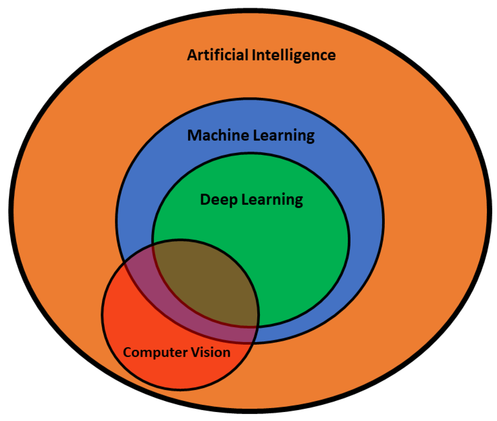
Artificial Intelligence (AI) is a field of computer science. Its goal is to create algorithms that mimic human intelligence to solve problems and automate decision-making [35]. AI research started in the 1940s and was focused on game solving, automatic mathematical proofs, automatic translation, etc. AI is currently used as a synonym for “Deep Learning” in media, but AI refers to many different sub-fields such as Automatic Game Solving, Natural Language Processing, Computer Vision, Logic Programming, Expert Systems, Data Mining, Intelligent Agent systems, robotics, Machine Learning, Deep Learning, etc.

These sub-fields are not mutually exclusive. For example, Machine Learning is used for Data Mining, Natural Language Processing, Computer Vision, Intelligent Agent systems, etc. Relationships between AI, ML, DL and Computer Vision are represented in Figure 1.

In this review, we focus on Computer Vision for grape-yield prediction.

2.2. Computer Vision and Machine Learning

Computer Vision refers to AI algorithms designed to extract knowledge from images or videos. Image-processing algorithms perform operations directly on the pixels with rules selected by human developers. However, natural images contain scenes that are too complex to be effectively processed in this manner. Another complexity is the large size of modern high-resolution images. There are too many possible variations to account for with this kind of image. The first solution is to apply constraints to the image acquisition environment with artificial backgrounds, centered objects, artificial lighting, etc.

Another solution is to use Machine Learning (ML). ML refers to algorithms that can solve tasks without being explicitly programmed by a human developer. Image processing algorithms and ML models are combined to solve complex applications.

Computer vision algorithms follow a generic framework with multiple steps:

• Preprocessing to make the following tasks easier. This includes image normalization, background removal, denoising, and feature extraction.
• Performing the main task of the application. This produces a raw output (like a classification score).
• Post-processing of the output to correct the raw output and make it interpretable.

The second step performs one of these tasks: image classification, object detection, or segmentation. Classification associates a class or category to an image. Object detection combines classification with location estimation; the detected objects are surrounded by bounding boxes. Segmentation goes one step further by performing classification of each pixel in the image.

Many ML algorithms are available. The simplest classification model is logistic regression. It is limited to data that can be linearly separated. Common ML models include Decision Trees, Support Vector Machine (SVM), K-Nearest-Neighbors (k-NN), and Multi-Layer Perceptron (MLP, also known as a feed-forward network), etc. ML models cannot be applied directly to raw images because (1) they do not exploit the topology images (connectivity of pixels), and (2) images have too many variables (one for each pixel and each channel). For example, a small red–green–blue (RGB) image of 10 × 10 pixels has 300 variables.

A technique known as feature extraction is applied to images to obtain the most relevant information into a small set of variables. An ML model is then trained and evaluated.

2.3. Deep Learning

Deep Learning (DL) refers to modern neural networks. Convolutional Neural Networks are an adaption of the MLP model with shared neurons represented by convolutional filters. This reduces the number of parameters and processing of pixel neighborhoods. Convolutional Neural Networks (CNN) were created by Yann LeCun in the late 1980s [36]. They were primarily designed for image classification, but they can also be adapted to time-series regression. CNNs are currently the state-of-the-art method for image classification because they are very effective at learning both the features and the classifier from the data. CNNs have been adapted to more complex applications such as object detection and image segmentation. These complex models use a CNN as a pre-trained backbone. This is known as transfer learning, and it allows the transfer of existing models to other applications. This is useful to compensate for a lack of training data.

Object detection models perform both classification and localization of objects in images. The model is trained to predict the coordinates of the boxes around the relevant objects. This can be done with two-step models such as Faster R-CNN [37] or R-FCN [38]. Other models have simpler architecture to perform detection in one step: Yolo [39], Single Shot Detector [40], RetinaNet [41], etc.

Similarly, CNNs have been adapted to image segmentation. A first approach uses a CNN for pixel-wise classification with a sliding window [42]. This approach is still commonly used with either CNN or ML models. However, pixel-wise classification is highly inefficient because it only produces one output for the central pixel of the input. The output could be applied to the whole input patch, but it would lower the accuracy by producing a coarse segmentation. A solution was proposed by Shelhamer et al. [43] with a Fully Convolutional Neural Network (FCN). This kind of semantic segmentation model is known as an encoder–decoder architecture. The encoder is responsible for automatic feature extraction. The decoder uses its output to produce a dense pixel-wise prediction. A popular architecture is the Unet model [44], which uses a symmetrical encoder and decoder.

2.4. Evaluation of Machine Learning and Deep Learning Models

ML methods have to be evaluated on multiple datasets to assess the generalization performance of the model (“Is it able to perform on new data?”). The evaluation of an ML method can be done by dividing the database into two parts: the training set used to create the model, and the validation set. This train/validation is random and, a third independent dataset, a test set, can be used to obtain better evaluation. Different performance metrics can be calculated on both datasets. The performance should be similar on both training and validation/test sets. A gap between training and validation/test performance may imply overfitting of the model (i.e., it cannot generalize correctly on unseen images). The most commonly used metrics are recall (ratio of detected objects), precision (ratio of objects detected among the predictions), F1 score or F-measure (harmonic average of the recall and the precision), and accuracy (ratio of correct predictions).

These metrics are calculated using the confusion matrix shown in Figure 2. Accuracy (Equation (1)), recall (Equation (2)), precision (Equation (3)), and F1 score (Equation (4)) are calculated for each class (most studies mention only one class: grapes, berries, or flowers). Accuracy can be skewed when one of the classes is under-represented in the database; in that case, the F1 score is preferred.

The framework presented in this subsection is generic—it can be applied to most computer vision applications. Grape-yield prediction needs a fourth step for occlusion modeling. Many fruits, berries, or whole grape clusters are hidden by foliage, by internal occlusion of grapes, and by one-sided image acquisition. Modeling generally uses regression techniques to estimate the number of hidden berries or to predict the yield. Regression metrics are then used to evaluate performance. This includes the Coefficient of Determination (or R-squared, R²), Mean-Square Error (MSE, Equation (5)), and Root-Mean-Square Error (RMSE, Equation (6)) or Mean-Absolute Error (MAE, Equation (7)), and Mean-Absolute-Percentage Error (MAPE, Equation (8)).

$$Accuracy=\frac{TP+TN}{TP+FN+TN+FP}$$

(1)

$$Recall=\frac{TP}{TP+TN}$$

(2)

$$Precision=\frac{TP}{TP+FP}$$

(3)

$$F1=\frac{2\times Precision\times Recall}{Precision+Recall}$$

(4)

$$MSE(\widehat{y},y)=\sum _{i=1}^n\frac{{({\widehat{y}}_i-y_i)}^2}{n}$$

(5)

$$RMSE(\widehat{y},y)=\sqrt{MSE(\widehat{y},y)}$$

(6)

$$MAE(\widehat{y},y)=\frac{1}{n}\sum _{i=1}^n|{\widehat{y}}_i-y_i|$$

(7)

$$MAPE(\widehat{y},y)=\frac{1}{n}\sum _{i=1}^n\frac{|{\widehat{y}}_i-y_i|}{{\widehat{y}}_i}$$

(8)

2.5. The Difficulty of Comparing Existing Yield-Modeling Work

The comparison of existing works is problematic for several reasons. First, existing works are limited to a few varieties at a specific moment and in different parcels across the globe. Therefore, many sources of variation can affect the results: variety, phenological stage, and location of grapevines. Second, the number of images and studied grapevines are sometimes very different from one study to another. The difficulty of acquiring data can explain this difference. Indeed, images can only be taken during a limited period of the year and potentially in a limited number of parcels. Labeling these images is yet another problem because this step is quite time-consuming. The acquisition of data such as the number of grapes and berries as well as their mass is limited by the available workforce. Therefore only a few studies cover multiple varieties on a significant number of grapevines over several years. Further, many works are carried out in totally or partially controlled environments to perform a specific measurement or to make processing easier. This includes artificial backgrounds used to detach the grapes from the images. Similarly, artificial lighting at night (or with a powerful flash) is often used, as the background is not visible in this condition. Artificial lighting can also be used to generate an easy-to-detect pattern on the fruits. The environment can also be controlled by defoliating the vine to simulate different foliage occlusion and vigor levels. The occlusion created by the foliage is currently the biggest limiting factor for yield modeling. An example of vines before and after defoliation is shown in Figure 3.

Finally, the last difficulty of this kind of comparison is the usage of different performance metrics. Consequently, there are no established standards that directly compare the performance of various grape detection methods and yield estimation.

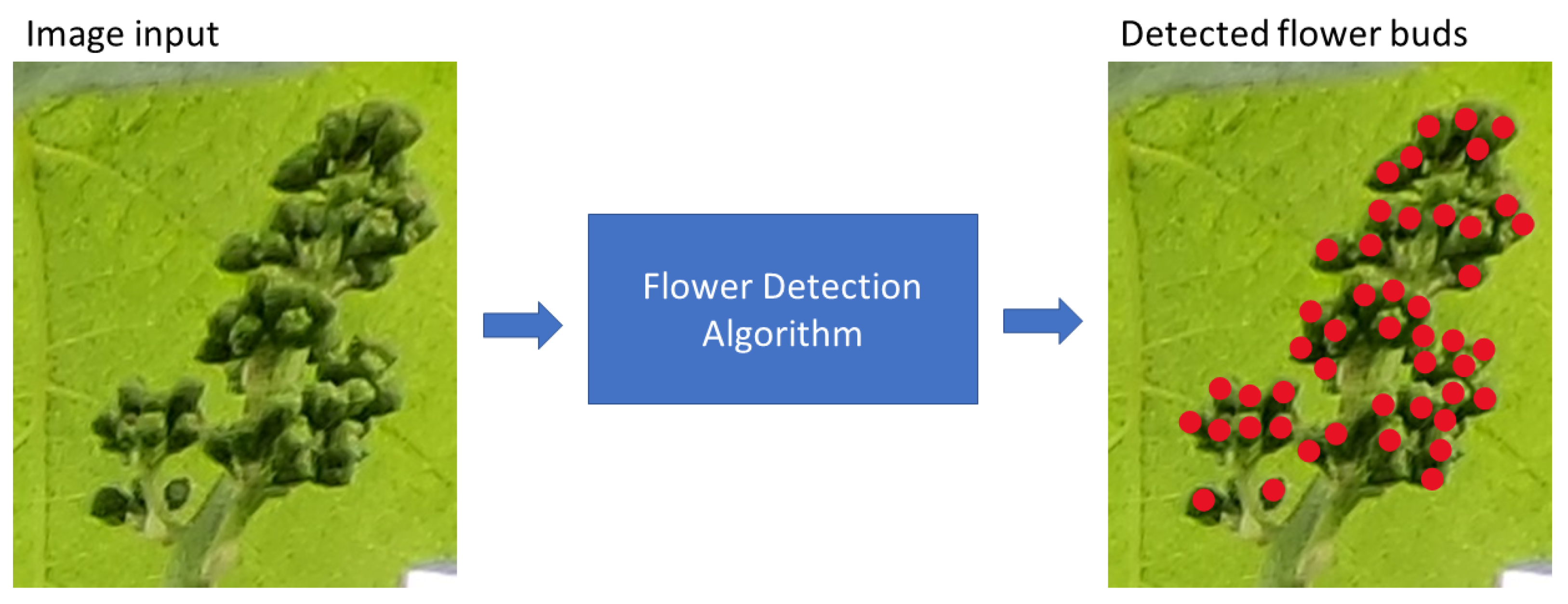
3. Flower Counting

The first application presented in this summary is the detection and counting of flowers (an example is shown in Figure 4). Counting is generally performed at the BBCH 55 stage, when the flowers are not separated and form small buds. The objective is to count the number of inflorescences (the future grape bunches) and the number of flowers (the future berries). Counting the flowers enables early prediction of the potential yield. It remains, however, an inaccurate prediction, because some flowers will fall (run out) during fruit setting. Thus, the problem of detecting flowers is closely related to the one of berry detection. Nonetheless, this task is more complex since flowers are small, approximately 3 mm in diameter, and have a green color similar to the foliage color. Several methods have been suggested, and most of them require partial control of the environment (artificial background or lighting) to simplify the task. The different approaches presented in this section are summarized in Table 1.

3.1. Classical Methods—Counting Using Key-Point Detection

A first approach consists of detecting flower-bud candidates and then filtering the detected elements to preserve only the true flower buds [45,46,47]. One commonly used detection criterion is the reflection pattern of light on the surface of the flower buds (this is also used to detect berries). When the flower buds reflect the light, they correspond to the local maxima of the image. They are detectable using algorithms such as the “h-maxima transform”, which detects every local maximum greater than a threshold h. There are, however, several obstacles to this detection, as the background of the image and the choice of the detection threshold may lead to several false positives. A simple way of removing the false positives caused by the background consists in using an artificial background with a single color (black in the case of flower detection). The use of a black background drastically simplifies the preliminary processing of the image, and even a simple segmentation method such as Otsu’s method [48] allows the removal of the background from the image. Further, false positives caused by the choice of the detection criterion can be removed using filtering methods. For instance, some authors [46,47] use the size, shape, and distance of the flower candidates as filtering criteria for images obtained against an artificial black background. The method proposed by [45] improves the method of [47] by using specific morphological operators to remove the natural background (an artificial background is therefore no longer necessary) and detect potential flower buds. The method proposed by [49] used a similar approach in the binary image only, where a morphological operator and a watershed algorithm were used to delineate the flower buds. Although it achieves a good counting correlation of R${}^2$ = 0.99, it does not compute the location of the flowers in the image.

Several weaknesses in the previous studies have been identified by [50]. The methods proposed by [45,46,47,49] all depend on manually chosen parameters (the size of the morphological operators, for example). Therefore, these methods are sensitive to the color and the apparent size of the flowers. In addition, the reflection pattern of the light used as a detection criterion is not robust and can strongly vary depending on the grape variety. As a consequence, one method has been proposed to correct these weaknesses [50]. The stems and inflorescences are detected with a segmentation algorithm that uses active contour propagation. The potential flowers are selected with the generic SURF key-points detection method. They are filtered with a non-supervised method, K-means, because the authors suppose that a supervised method would not be robust enough to variations caused by natural lighting [51]. Analysis of the impact of the phenological stage shows that detection performance is constant after the agglomeration of the flower buds (stage BBCH 55). More recent studies have applied particle analysis for flower detection [52]. This method has the same weaknesses as the previously mentioned studies because the apparent size of the flowers must be defined in pixels. In addition, the work of [50,52] does not address the issue of segmenting the background, and therefore requires an artificial black one.

3.2. Deep Learning and Performance

To this day, multiple DL methods have been suggested for counting flowers. The published work by [53] uses a Fully Convolutional Network (FCN) segmentation model. One of the advantages of the FCN is its simplicity; the training process lets the model automatically learn the best features for the desired task. A large quantity of labeled images is necessary to train these models. Labeling is a time-consuming manual task. Tools have been developed to partially automate labeling. In the case of semantic segmentation, a first mask can be created by generating super-pixels or by watershed segmentation. These tools help save time, but the task is nonetheless painstaking because DL requires at least tens or hundreds, sometimes thousands, of high-quality images. An FCN model was used by [53] to detect inflorescences in images taken in natural conditions. This method allows the suppression of the image background. After this, the Hough transform is used to detect the flowers. The authors of [54] proposed a similar method with a SegNet [55] model for inflorescences segmentation in images of six varieties taken at night with artificial lighting. They studied three flower-counting methods on the segmented images: flower segmentation with the SegNet model, Watershed segmentation, and linear regression with the number of segmented pixels as a predictor. A similar FCN model proposed by Grimm et al. [56] has also been applied for the detection of flowers in natural conditions. The model detects flowers directly (represented by dots in the labeled masks) without a second step for counting. The object detection model Mask-RCNN has also been applied to flower counting [57]. It was evaluated on images of individual inflorescences with artificial backgrounds (dataset published by [50]).

The Mask R-CNN model proposed by [57] achieved better performance than the method of [50] on the same dataset, with up to a 98% F1 score on Chardonnay and an average of 6.92% MAPE counting error on all varieties. Performance was similar on four varieties on three different dates. More experiments are needed to assess the model’s counting ability in images with multiple inflorescences and natural backgrounds. The performance of the methods in [50,56] are similar, with an 84.3% success rate and an 86.7% F1 score. The method of [56] has the advantage of working directly in natural conditions, but the evaluation performed by [50] seems more robust (cross-validation over 12 databases). The method of [56] also requires a high-performance GPU for training and for efficient prediction, and between 4 and 8 s of execution time is required per image (this information is not specified by [50]).

Similar performance was achieved with the methods from [45], with 85% recall and 83.38% precision; [46], with 86% recall and 84% precision; and [52], with between 12.3% and 18.4% counting error. A lower score was achieved with the method of [47], with only 74.3% recall and 92.9% precision. The lower performance of [47] is caused by the complexity of the natural images (the background is artificial, but the lighting is natural) and the lack of robustness of the detection method (other studies use a more robust but more complex method). These two methods also have the downside of using manually selected parameters, rendering them sensitive to scale variations (the pixel size of the flowers must be known).

The DL method proposed by [53] seems limited by the performance of the Hough transform. Counting only obtains a 75.2% F1 score with the result of the segmentation, which only rises to 80% on the ground-truth masks. Combination of the segmentation model and a robust algorithm, such as the one proposed by [50] for instance, would perhaps improve the performance and be usable in real conditions. The methods proposed by [54] achieved up to 0.73 and 0.71 F1 scores with SegNet counting and Watershed counting. This is slightly worse than the method of Rudolph et al. [53], despite control of the background (image taken at night with artificial lighting). This could be explained by the occlusion caused by different varieties. Some varieties have bigger flower buttons that lead to higher occlusion. Another difference compared to other work is the use of automated image acquisition from a vehicle. This was designed to take images of whole vines; therefore, some inflorescences can be out of focus (blurry), and flowers can have a smaller apparent size than with manually taken images.

Table 1. Comparison of different approaches for counting flower buds.

Approach	Material	Techniques	Results	Comments
Local maxima and circle detection [45,46,47,49,52]	132 images, 11 varieties, BBCH 53–57 stages, artificial background [46]	H-maxima transform [46].	85% F1 [46].	Requires calibration and uniform background [46].
Generic key point detection [50]	533 images, 4 varieties, BBCH 18–61 stages, artificial background	Detection and filtering	84.3% accuracy.	Requires uniform background.
Deep Learning [53,54,56,57]	30 images, 2 varieties, BBCH 73 stage, natural conditions [56]	FCN [56]	86.7% F1 [56].	Requires a powerful GPU [56].

Table 1. Comparison of different approaches for counting flower buds.

Approach	Material	Techniques	Results	Comments
Local maxima and circle detection [45,46,47,49,52]	132 images, 11 varieties, BBCH 53–57 stages, artificial background [46]	H-maxima transform [46].	85% F1 [46].	Requires calibration and uniform background [46].
Generic key point detection [50]	533 images, 4 varieties, BBCH 18–61 stages, artificial background	Detection and filtering	84.3% accuracy.	Requires uniform background.
Deep Learning [53,54,56,57]	30 images, 2 varieties, BBCH 73 stage, natural conditions [56]	FCN [56]	86.7% F1 [56].	Requires a powerful GPU [56].

4. Grape Detection

The second application presented in this study is the detection of grape clusters. The detection algorithm’s input is an image with grapes, and the output is an image containing the location of the grapes as well as their number (see Figure 5). The different approaches used for grape detection are summarized in Table 2.

This is an important step because it enables several practical applications such as yield estimation, automatic harvesting using a robot [58,59,60], automatic spraying of growth hormones [61], and characterization of phenotyping [62]. This task is potentially difficult for multiple reasons: (i) there are several factors of variability (lighting, distance, and complex background) in natural images, (ii) occlusion created by the foliage, and (iii) color confusion between the grapes and foliage.

4.1. Segmentation Using Thresholds

A simple approach consists of thresholding segmentation. One or more thresholds are chosen to be applied to the pixels to keep only the areas that correspond to fruit. Thresholding segmentation is a simple approach that was first used by [63] to evaluate the potential of image processing for yield estimation. Thresholding segmentation algorithms usually have short execution times and are easy to develop. However, these algorithms have several drawbacks that limit their use in the field without partial control of the environment. The main issue is that strict thresholds are not robust to the color variations caused by natural lighting and the background. The images taken by [63] contain only easy-to-detect red grapes in a fixed frame. They have been applied in field on red and white varieties but only during the night and with artificial lighting [58]. They have also been studied in laboratories [64] and controlled environments with artificial backgrounds [65]. A better thresholding approach consists of using the Mahalanobis distance to compare the pixels in the image to reference pixels representing various classes. The predicted class of a pixel is then chosen by selecting the one with the smallest Mahalanobis distance. This technique has been used to detect grapes and to estimate leaf area [66], porosity, and exposure of the canopy and the grapes [67]. In both cases, a controlled environment with an artificial background or a lighting system at night is necessary. Therefore this method requires controlled conditions to prevent variations in lighting and background. Moreover, the thresholds must be determined in each situation. This technique is appropriate for studies in laboratories or in the field with a vehicle designed for phenotyping [16]. It can also be employed in natural conditions in more straightforward situations, such as the detection of red grapes from UAV images after defoliation [9,68]. However, the grapes must have attained the maturity to discriminate their color from the ground or the leaves. To conclude, with this approach, it is possible to automate segmentation using a non-supervised classification algorithm such as Fuzzy C-Means or K-Means [69,70]. The false positives are then filtered with a Support Vector Machine (SVM) classifier. This method remains sensitive to lighting changes and has only been evaluated on red varieties.

4.2. Edge-Based Segmentation

A second approach uses more complex segmentation techniques. Active edge segmentation has been proposed to detect white grapes for automated harvesting [71]. It is limited in its use to nighttime with a lighting source, which erases the background elements (sky, ground, and further rows). The authors of [61] suggested a hybrid method combining a binary threshold and edge detection. More specifically, it uses the density of the edges in the image as a criterion to detect grapes. However, this method requires manually identifying several parameters (size of the convolutional filters, thresholds, etc.) to function correctly. The thresholding segmentation technique can be combined with other pieces of information, such as depth, to achieve better results. Depth manages to more easily discriminate the foreground from the background. The work of [72], therefore, combines depth maps, built using stereoscopic images, analysis of the edges, and color-based segmentation. This technique has been evaluated in natural conditions but only on red varieties, a condition that makes grape detection easier.

4.3. Pixel Classification

A third approach uses ML to make the detection of grapes more robust to lighting variations. It segments the image by using small pixel neighborhoods, or blocks, as inputs for a classification model. Examples of pixel neighborhoods are illustrated in Figure 6.

The model produces a binary output (grape or non-grape) that is applied to the central pixel or the entire input block. Classical ML techniques cannot be directly applied to raw images, as features must be extracted first for each block. A simple feature is the mean values of the R, G, and B channels to produce a vector with only three components. In practice, numerous methods are available and have been applied to this problem. This approach was proposed in 2006 by [73] for automated grape harvesting. Zernike moments, a set of invariant descriptors, have been used as features to train an SVM classifier. The mean value of the RGB channels has been used in several studies [74,75,76]. A genetic algorithm was suggested to select the best color channels among several possible color spaces (RGB, HSV, or CIELab) [77]. Another easy characteristic to calculate is the color histogram, although this technique is limited to controlled conditions [78]. More complex methods, such as a local structure tensor associated with a Bayesian classifier, allow for the segmentation of grapes and foliage in field conditions (natural background with flash for uniform lighting) [79,80]. More recently, CNNs have been used to combine the feature extraction and classification steps [81,82,83].

The choice of extractors is important because the quality of the features impacts the final results. In contrast, the choice of the classification method is less influential, as good results can be achieved with an SVM or Multi-Layer Perceptron (MLP).

In addition, pixel classification suffers from several limitations, including sensitivity to color (variety) and potentially long execution time. Execution time can be reduced, but it requires extra effort in optimization. Finally, the evaluation of this approach is often limited, and it is therefore not representative of actual performance. Evaluation is performed in two ways: by calculating either the performance for the classification of the blocks or the grape detection. Nevertheless, some studies only contain block classification performance [77,84]. In practice, performance above 95% can be obtained using block classification, but this is rarely observed when applied to entire images. A difference of approximately 3% is, for example, achieved by the method of Luo et al. [75] with a 96.56% success rate on the blocks, but with a 93.74% detection rate for individual grapes.

Optimization to reduce the execution time are also possible. The work of [85] proposes a two-step segmentation: (1) use of a logistic regression model to classify the pixels into seven classes, and (2) filtering of the false positives for the “grape” class using a bag-of-words model with SURF descriptors and an SVM classifier. Using a simple classifier directly on the pixels dramatically reduces the execution time and limits the usage of the SVM model to a reduced area of the image. This method has only been tested in a controlled environment: red variety and artificial lighting during the night. Further, the method proposed by [85] has several limitations: it only exploits the neighborhoods of the pixels in a small area (no more than a few tens of pixels) and is strongly dependent on the method used to extract features. For instance, some features solely work on red varieties (which are easier to discriminate from the foliage).

Finally, this approach can be used for 3D reconstruction of vines using stereoscopic images or structure-from-motion methods. As the objective is to classify 3D points instead of 2D pixels, feature extraction is more complex because it must take into account the depth of the objects. The 3D reconstruction could allow more precise characterization of grapes by estimating their size, volume, compactness, etc. The work of [86] uses a structure-from-motion method that generates a 3D reconstruction using a sequence of images and an SVM classifier. The authors of [62] use a stereoscopic camera and an Import Vector Machine classifier—an improved SVM—to detect grapes at night with artificial lighting. Even with the controlled environment, the proposed method only reaches an 82% detection rate at best. This performance can be explained by the chosen feature extractors and the classifier. Furthermore, it requires 10 GB of storage space and up to eight hours of calculations for 25 m of vine row, rendering it impractical without optimization and/or distributed computing.

A 3D reconstruction can also be achieved using video taken by a single-lens camera such that the reconstruction is based on movement to estimate the 3D position of objects (similar to structure-from-motion). The Simultaneous Localization And Mapping or SLAM method has been studied to estimate the volume of grapes and infer the size of the berries in a partially controlled environment (natural background and lighting with defoliated vines) with a 93% success rate [87]. The results of this method are better than the results of Rose et al. [62], but the wind can negatively impact it: objects must remain still in the analyzed sequence.

ML can also be used in another fashion. A similar approach to the one presented in the previous section tries to identify potential berries with a classification model that can be generalized to detect grapes. One advantage is that it reduces the number of calculations by suppressing many unnecessary pixels. This model has been used in the field on white grapes [88] and requires a relatively complex algorithm combining key-point detection, classification, and clustering. It has also been applied to red grapes [89]. Nevertheless, this method suffers from the same limitations inherent to methods that employ a feature extractor and ML. It is also more complex because the potential area detector method must be good enough to retain as many true positives as possible before filtering. Overall, we consider these methods complex because they mix different algorithms that require fine-tuning to operate.

4.4. Deep Learning

DL has recently been applied to the problem of detecting and counting grapes. A naive approach uses the same pixel-wise classification discussed previously, but with a neural network that combines both feature extraction and classification [81,83,90].

The use of CNNs greatly simplifies the detection step because the model learns the best features from the data. However, this method is always limited by the small size of the blocks and the long calculations required to segment one image. Several CNNs have been studied to predict the masses of grapes automatically [91]. The prediction error is relatively low, 11%, in controlled conditions with an artificial background, but the proposed method has many drawbacks. The distance between the grapes and the camera varies, impacting the results. This limit could be overcome using a depth sensor, but this approach should also be evaluated on several rows and with different varieties to better appreciate its potential.

Several popular object detection models, Faster R-CNN [37], R-CNN [92], R-FCN [38], and SSD [40] have been tested on the task of grape detection and counting using videos [93]. SSD was applied to grape detection at two stages (0.5 cm berries and 1.2 cm berries) in natural conditions and with real-time hardware acceleration (TPU) [94]. A Mask R-CNN model [95], which detects objects and segments them, has also been applied to the detection of grapes [96]. The counting of grapes from videos is corrected with a structure-from-motion method that estimates the 3D position along the camera path. The 3D position is used as an identifier to avoid counting one grape twice. Mask R-CNN and multiple Yolo models [39] were compared on the dataset published by Santos et al. [96,97]. Yolo models were also compared on red grape detection from smartphone images [98]. A Faster R-CNN model was applied similarly, with a tracking algorithm to process videos of Riesling and Pinot Noir vines taken at night with artificial lighting [99]. Mask R-CNN has been studied in multiple recent works [100,101,102]. The authors of [100] compared the performance of Mask R-CNN to other models such as U-Net and Yolov3 [103] (they also used the WGISD benchmark published by Santos et al. [96]). They found better precision with U-Net and better recall with Yolov3. The authors of [101] applied Mask-RCNN to the GrapeCS-ML dataset published by Seng et al. [32]. It contains images of different varieties taken in natural conditions at different stages. One limitation of this dataset is that most images only contain one grape cluster, so the resulting model cannot process images with many clusters.

Mask R-CNN was also applied to stereo-images to detect and reconstruct 3D models of grapes for automated harvesting [102]. A Yolov4 [104] model was applied to low-resolution images of white grapes to measure the correlation between grape counting and fruit weight [105]. Low correlation was found between the number of detected clusters and the actual number of clusters (R${}^2$ = 0.24). The correlation between the number of detected clusters and fruit weight was better (R${}^2$ = 0.59), indicating a potential application for yield estimation in future work. Further, the SDCNet model, initially developed for crowd counting, was applied to bunch counting in omnidirectional images of Delaware grapes, reaching a counting error superior to 10% NRMSE.

Chen et al. proposed a modified PSPNet [106] model for grape segmentation [107]. It was applied on white and red grapes after veraison. They reached good segmentation performance, with an average of 87.42% IoU. Similar results were obtained on both red and white grapes. However, the main limitation of semantic segmentation models is their inability to separate overlapped clusters. This result in inaccurate grape counting. Similarly, the authors of Peng et al. [108] applied a DeepLabV3+ model to multiple red, green, purple, and black varieties, with or without spherical berries. They reached an IoU of 88.44% with an inference of 60 ms/image, which allows automatic harvesting. The authors are well aware of the difficulty of separating overlapping grapes and proposed the use of a depth sensor (Intel Realsense D435 stereo camera) to solve this problem [109]. Their results, 85.6% recall and 87.1% precision, show the viability of their solution. However, this method should be compared to object detection models.

Finally, a generative model was proposed to adapt images to different lighting conditions [110]. A CycleGAN [111] model was used to translate images taken in daylight to images taken at night with artificial lighting. This step can be useful to increase the size of existing datasets and make the models robust to varying environmental conditions.

4.5. Performance Comparison

Regarding performance, thresholding segmentation is difficult to apply in real situations unless heavy constraints are used, such as artificial lighting at night [58]. In these conditions, 91% of white grapes and 97% of red grapes are detected. However, this method remains limited by the thresholds that have to be selected for each situation. The method of [66] shows high counting performance with a 98% success rate. However, this performance should be considered cautiously because the evaluation was only performed on ten vines that were progressively defoliated to acquire more images. The performance achieved by Diago et al. [67] are close to those of Reis et al. [58] with a 92% F1 score. Both these methods require artificial lighting at night or artificial backgrounds. The detection rate of the method developed by Berenstein et al. [61] nears that of the previous methods at 90% but with a high false positive rate of 70%. Similar performance has been seen in the methods of Xiong et al. [71], with a 91.67% success rate, and Correa et al. [69], with a 95% success rate. A mean classification precision of 89% was achieved on the pixel level with multi-spectral imaging in natural conditions and multi-step segmentation with K-means clustering. However, the results are limited by the small number of images used for validation (only six) and the limited practicality of the acquisition device (slow and expensive). Overall, this approach is generally limited to controlled-environment studies rather than real situations such as the study of the correlation between pixels belonging to grapes/masses [63], comparison of 2D and 3D detection methods [64], or estimation of the number of hidden grapes [65].

The second approach can be used in partially controlled environments. The method proposed by Chamelat et al. [73] nearly achieves a 100% success rate but was only evaluated on 18 low-resolution images. A detection rate of approximately 94% of red grapes in natural conditions wass presented by Luo et al. [75]. A similar detection rate of 93% was reached by a simple pixel classification method [74]; unfortunately, the performance on white grapes was not as good. Recall of 85% and precision of 93% were attained by Abdelghafour et al. [80] on a red variety before ripening and with a flash. This is an improvement on their previous work [79]. Performance can vary greatly depending on the selected techniques and the conditions in which the images were taken. A detection rate of 90% was obtained on images taken during the night with artificial lighting and containing very visible red grapes. A high success rate of 99% was attained by the method proposed by Behroozi-Khazaei and Maleki [77], but this only refers to the classification performance on a set extracted from the learning set of the classifier. The method has not been tested on full images, and the number of blocks used for creation and evaluation was limited and was achieved with a flash, a technique suitable for practical use. The method proposed by [88,89] are potentially less efficient because it depends on the precision of the preliminary segmentation (or detection of key points) method that is used. The detection rate reached by [89] remains, nonetheless, high, at 90%, in natural conditions; however, it was only tested on red varieties.

The method proposed by [88] achieved only an 80.34% recall rate (with a good precision of 88%) but has the advantage of having been evaluated on several databases with red and white grapes and in natural and controlled conditions (lighting at night). This performance, lower in comparison with other studies, can be explained by the more exhaustive validation method and by the complexity of the proposed method. An F1 score of around 80% was reached by the method of [85]. Finally, the 3D reconstruction method of [86] generates good results in natural conditions with an Area Under the Curve (AUC) ROC of 0.98 before veraison and of 0.96 after. However, the execution time of the method is not specified.

For DL, Mask R-CNN attained a 90% F1 score in natural conditions and without artificial lighting [96]. A similar score of 91% was obtained on the GrapceCS-ML dataset [101]. The Yolov4 model reached 96.96% mAP on the dataset published by Santos et al. [96,97]. They contributed to this dataset by labeling the individual berries. Yin et al. [102] reported an F1 score of 94.7% in ideal conditions (defoliated with front lighting). The worst performance was obtained with back-lighting, with an 86.7% F1 score. The best performance was achieved by [93] with 99% average precision in real conditions. Few details about the data used in this work are available, so better performance could be expected on defoliated vines near the harvesting date.

The Yolo model proposed by Li et al. [98] reached similar results, with a 95.62% F1 score on both green and red varieties. Images were taken with natural lighting but with well-visible grapes from partially defoliated vines. This is representative of the expected condition for automatic harvesting. For this purpose, their model reached an inference time of only 12 ms per image on an Nvidia GTX 1050Ti GPU. Similarly, a counting error of 13.3% was reported in the work of Sozzi et al. [112] with a Yolov5x model. The performance obtained by Aguiar et al. [94] seems to be closer to the natural condition of many vineyards: their SSD-MobileNet model reached 49.85 and 53.34% mAP on grapes before veraison, without defoliation, and at two different phenological stages.

Jaramillo et al. [99] reported a maximum counting error of 12.5% with a similar method in images taken at night with artificial lighting. The good performance was achieved early in the growth stage when the foliage had developed enough to cause massive occlusion of the fruit area. It was also shown that the maximal error of manual counting, 23.5%, was much higher than that of the proposed method. Occlusion caused by foliage is a source of error for object-detection models. They are not able to detect small clusters that are partially hidden by leaves. Both object-detection models and segmentation models can achieve good performance on defoliated vines [100], with up to 92.7% F1 score on the grape pixel area. Another source of error is the difficulty of counting overlapping clusters; a method was proposed to solve this problem for the case of two overlapping clusters, but there is no method yet able to count an arbitrary number of overlapping grapes [60].

A 99% success rate was also shown by [81], but it was only on blocks extracted from images for pixel-wise classification. Similar methods proposed by [82,83] achieve a 91.52% success rate for the counting of grapes and an 80.58% success rate in segmentation. These three methods do not harness the full potential of DL because they only use classification models. This can be explained by a lack of computing power and RAM. Indeed, a block-wise classification method requires less computing power and RAM than a specialized method for semantic segmentation. Nonetheless, these methods can obtain good performance and are capable of distinguishing between green grapes and leaves in some conditions (natural lighting, natural background, and well-calibrated distances and angles). We have shown in previous work [113] that better performance can be achieved with a fully convolutional network such as U-Net by allowing segmentation over uncalibrated images of white grapes. Our comparative study showed that pixel-wise classification is limited by its small input size and by the unbalanced nature of the vine images (the fruit area represents only a small part of the image).

Please note that computing power and the quantity of labeled data are the main limitations of the use of DL. Most databases are not sufficiently large, requiring artificial data augmentation through the use of random transformations on the original images to create new samples. Moreover, convolutional neural networks applied to images require a powerful GPU accelerator so that the training process can be done in a reasonable amount of time. A powerful CPU and GPU are needed to train a DL model with image augmentation. Some 3D reconstruction methods also need high-performance computing or specific optimizations [62].

It should also be noted that data augmentation can results in biased performance measurement if it is not done properly. Data augmentation can be done in two manners: (1) online by generating augmented mini-batches during training, or (2) offline by oversampling the training set. Offline augmentation was performed by many works presented in this review [94,98,107]. It can lead to data leakage if the train/validation/test split is performed after offline augmentation. This is the case in the work of Zhang et al. [114] (10-fold oversampling before splitting).

The detection of grapes could be a preliminary step for more specific tasks. For automatic harvesting, detecting the location of the cutting point is also necessary. This additional step generates difficulties because the grapes must be individually separated, whereas some grapes overlap in the image. A method has been suggested to solve this problem with two grapes [60]. The segmentation of grapes and leaves has been applied to optimize the use of pesticides and growth hormones [61]. This study shows that targeted spraying could reduce the quantity of pesticides by 30%. Grape detection and 3D vine reconstruction are currently being used for phenotyping by estimating multiple traits of the vines, such as the diameter, volume, or size of the berries or grapes, at a large scale. In practice, stereoscopic 3D reconstruction is not practical at an industrial level because it requires massive computational resources [16,62]. The detection of grapes is also the first step toward yield estimation. The number of grapes must be turned into a yield estimation. Preliminary studies have evaluated visual estimation methods of the mass of the grapes in the laboratory with a 5% error rate [78], in the field with a correlation of R${}^2$ = 0.87 [64], and using DL with an 11% error rate [91]. This visual estimation method is not satisfactory because it strongly depends on the distance between the camera and the fruit. The following section presents existing berry counting methods.

Table 2. Comparison of different approaches for grape detection.

Approach	Material	Techniques	Results	Comments
Thresholding [9,16,58,63,64,65,66,67,70,78].	190 images, artificial lighting at night [58].	Color-based thresholding [58].	97% and 91% accuracy rates on white and red varieties [58].	Not suitable for daylight processing in natural condition [58].
Edge-based segmentation [61,69,71,72].	951 images, white variety [71].	Active contour segmentation [71]	91.67% accuracy [71].	Not suitable for daylight processing in natural condition [71]
Pixel classification [68,73,74,75,76,77,79,80,81,82,83,85,89,115].	200 images, red variety, natural conditions [75].	Color features and AdaBoost [75].	93.74% accuracy [75]	Inefficient, performance limited by the small input [75].
Region-of-interest detection and filtering [88,89].	163 images, natural conditions, red and white varieties, after ripening [88].	Key-point detection, classification, and clustering (SVM and Density-Based Spatial Clustering of Applications with Noise) [88].	84% F1 [88].	Careful calibration needed (detection algorithms, parameters, etc.) [88].
3D reconstruction and classification [62,86,87].	25 Riesling vines (white), stereo-camera, at night with lighting [62].	3D reconstruction and classification of 3D points [62].	80% F1 [62].	First step toward large-scale phenotyping, further optimizations are needed (execution time, memory requirement) [62].
Deep Learning [81,83,84,91,93,94,96,97,98,99,100,101,102,105,107,108,109,110,112,116].	300 images, five red and white varieties, natural lighting [96].	Mask R-CNN [96].	91% F1 [96].	Requires powerful GPUs and many labeled images [96].

Table 2. Comparison of different approaches for grape detection.

Approach	Material	Techniques	Results	Comments
Thresholding [9,16,58,63,64,65,66,67,70,78].	190 images, artificial lighting at night [58].	Color-based thresholding [58].	97% and 91% accuracy rates on white and red varieties [58].	Not suitable for daylight processing in natural condition [58].
Edge-based segmentation [61,69,71,72].	951 images, white variety [71].	Active contour segmentation [71]	91.67% accuracy [71].	Not suitable for daylight processing in natural condition [71]
Pixel classification [68,73,74,75,76,77,79,80,81,82,83,85,89,115].	200 images, red variety, natural conditions [75].	Color features and AdaBoost [75].	93.74% accuracy [75]	Inefficient, performance limited by the small input [75].
Region-of-interest detection and filtering [88,89].	163 images, natural conditions, red and white varieties, after ripening [88].	Key-point detection, classification, and clustering (SVM and Density-Based Spatial Clustering of Applications with Noise) [88].	84% F1 [88].	Careful calibration needed (detection algorithms, parameters, etc.) [88].
3D reconstruction and classification [62,86,87].	25 Riesling vines (white), stereo-camera, at night with lighting [62].	3D reconstruction and classification of 3D points [62].	80% F1 [62].	First step toward large-scale phenotyping, further optimizations are needed (execution time, memory requirement) [62].
Deep Learning [81,83,84,91,93,94,96,97,98,99,100,101,102,105,107,108,109,110,112,116].	300 images, five red and white varieties, natural lighting [96].	Mask R-CNN [96].	91% F1 [96].	Requires powerful GPUs and many labeled images [96].

5. Berry Counting

The counting of grape berries is one method currently used to perform yield estimation. Grapes are harvested from random samples to estimate the number of grapes per vine, the number of berries per grape, and the weight of the berries. These yield components make up, respectively, 60%, 30%, and 10% of the yield variance [117]. They are used in a yield equation that is applied to the entirety of the parcel to estimate or predict kg/ha (or kg/vine, hL/ha, etc.). This method is destructive, as the grapes must be harvested, limiting the sample size. This limit makes the predictions vary greatly depending on the year and parcel. Several studies proposed methods for automatic counting of grapes by computer vision. The main approaches for automatic berry counting from images are presented in the summary of this section in Table 3. Berry counting is illustrated in Figure 7. A rapid count can be obtained in the laboratory with a scanner [118] or with a camera and an artificial background [119], although this still requires destructive sampling. The first method that could be applied in the field was proposed in 2010 and was based on the detection of ellipses [120]. The proposed sensor was limited to a single grape cluster per image with an artificial background. The counting results were disappointing, showing a 30% success rate, mainly because the berry edge extractor generated too many false negatives.

5.1. Counting by Key-Points Detection

Numerous counting methods have been suggested. They consist of firstly detecting the berries and then deducing the number of grape bunches (which corresponds to 90% of the variance in the yield). The problem can be formulated as a circle detection or local maxima detection task. Specular reflection, caused by the light on the surface of the berries, produces a pattern that follows a Gaussian distribution. The berries appear as bright little spheres, which makes them more easily distinguishable from the background of the image. One of the first methods exploiting specular reflection used a Gaussian kernel to process images taken with a smartphone with flash [121]. It was limited to close-up images of one or several grapes to limit confusion caused by the background. Similarly, a morphological operator was designed to detect this pattern. It can only be applied to images taken at night with artificial lighting to produce the reflection pattern and to erase the background [122].

Several algorithms have been used to detect berries: the h-maxima transform [123,124], the fast radial symmetry transform [125,126], and the Hough transform [127,128,129,130,131,132,133]. The fast radial symmetry transform detects berry candidates rapidly, whereas the Hough transform potentially has high memory usage and computing power needs; it is also sensitive to noise. An alternative to the h-maxima transform, named invariant maxima detector, was proposed by Nuske et al. [125] to detect berry candidates with artificial lighting. These studies show that detectors based on local maximums are too sensitive to variations in natural lighting, making the use of a flash or lamp a necessity. The artificial lighting creates a uniform specular reflection on the surface of the berries, making the detection easier.

This technique also requires an additional filtering step similar to the one explained in the previous section. This classical approach is therefore complex because it requires several algorithms that need to be fine-tuned to (1) detect the berry candidates, (2) extract the features of each candidate, and (3) filter the false positives with a classifier. Therefore, it requires three separate algorithms selected among numerous existing methods.

The choice of candidate detection method is crucial because this step strongly impacts the final detection number. Thus, the algorithm with the highest detection rate must be chosen without worrying about false positives.

Feature selection is the most important step to distinguish the berries from the background and the foliage. The features should not be based solely on colors to avoid confusion between berries and leaves. Indeed, features representing the edge of the shape are most often used, as this allows the detection of berries without using an artificial background.

Finally, the choice of the classifier is less important, because similar performance can be achieved with classical models such as an SVM or an MLP if the extracted features have enough discriminatory power. Several classifiers have been studied: SVMs [88,115], K-nearest-neighbors [134], MLP [123,124,135], random KD-Forest [125], and convolutional neural networks [84,133]. A high success rate, close to 100%, can be obtained with a CNN. A CNN can be trained easily because it only uses small pixel windows, about 10 × 10 pixels, as input. We may also cite the work of [136], which proposed a reversed approach. In that work, the grapes were first detected using the Mahalanobis distance, and the segmentation was later refined with special filters. Finally, a Boolean model detects the berries. The Boolean model is more robust to obstructions because it is capable of detecting partially hidden berries. However, this method requires a controlled environment (artificial lighting at night).

The circle detection method can also be used for the 3D reconstruction of the grapes. The goal is to detect spheres amongst a cloud of 3D points. The Hough transform can be applied in three dimensions for this purpose [137]. This approach was evaluated on 100 vines in very controlled conditions (laboratory with four lamps and an artificial background). Despite these conditions, the proposed method only reconstructed 20% of the berries autonomously. Manual calibration was necessary for correct 3D reconstruction. It was also applied in the field [62,138]. The method of [138] compares estimates of the volume, weight, and number of berries with an automated reconstruction found using a semi-automatic method (human intervention is required). The automatic estimation method is competitive with the semi-automatic one, but precise calibration is necessary in both cases. Moreover, this method is potentially expensive because it uses five cameras. This approach detects berries in the field as long as the lighting is controlled with an artificial source, although the use of an artificial background is not essential in this case.

5.2. Deep Learning

DL can simplify berry counting by processing raw images. CNNs can be used as a feature extractor and as a classifier at the same time to filter berry candidates. This technique has been implemented on a Raspberry Pi [133] for real-time detection. CNNs have also been shown to be more accurate than SVM [84]. Furthermore, CNNs have been adapted to object counting with density map prediction. The areas with strong density correspond to the berry locations [139]. This method manages to count berries with an error rate of approximately 10%. CNNs have also been adapted to image segmentation. These CNNs have shown very promising results. An FCN model was proposed to count berries with two classes of labeling: the inside of the berries and the edges [140]. The model is faster and better than Mask R-CNN [95] and UNet [44]. This difference is explained by the structure of the models, as Mask R-CNN uses a complex structure to detect and segment objects, and by the small size of the database. Deng et al. [97] used the Hough transform for circle counting after grape detection with the Yolov4 model (it is similar to the method proposed by Rudolph et al. for flower counting [53]). One limitation of this algorithm is its sensibility to berries’ apparent size (the radius must be known). A Hybrid Task Cascade model, an improvement of the original Mask R-CNN model, was applied to berry detection for assisted grape thinning with smart glasses [141]. Simulated grape thinning was proposed as data augmentation to reduce the number of misclassifications. Therefore, this method was designed for processing in natural conditions but with a single grape bunch taking most of the image area. Worse performance may be expected on whole vine images. Miao et al. proposed edge detection to solve the problem of counting overlapping berries [142]. The proposed methodology is complex, with a Holistically-Nested Edge Detection model for berry edge segmentation, a Yolo model for berry detection, and a RANSAC algorithm for sphere fitting. It was evaluated on images of individual grape clusters in different conditions (laboratory or field conditions). A simpler object detection model based on RetinaNet [41], modified with a counting section, was evaluated on three plants for counting bananas-per-bunch, spikelets-per-wheats-spike, and berries-per-grape-cluster in natural conditions [143].

Palacios et al. recently proposed a three-step segmentation process with SegNet models for grape, berry, and canopy feature extraction from images taken at night with lighting. The goal is to use segmentation to measure traits with predictive power for actual berry counting (visible + hidden) with regression models.

5.3. Performance Comparison

Encouraging results were achieved by [56]. A single segmentation model was evaluated on several tasks, including berry, flower, and branch counting. It obtained good results with natural lighting, with or without an artificial background. Moreover, better performance was achievable by optimizing the structure of the model depending on the considered task and by using more images (only 60 images of red grapes were used). This model also uses a simple binary segmentation (each berry is represented by a point in the labeled mask). DL, Mask R-CNN more precisely, was combined with a SLAM 3D reconstruction technique to count berries in real-time [144]. A blower was used while taking the images to remove the leaves. The performance was impressive, with 96.62% precision and 98.81% recall on a row of 187 m. Similar results were obtained by Buayai et al., with 96.55% correct detection and only 2.79% misclassification error on images of individual grape bunches. Similar performance was also achieved with a multi-step berry counting model, with a recall of 96.24% and precision of 94.65% [142]. One limitation of this method is the need for high-quality edge labeling, which is time-consuming. It is also limited to images of individual grape clusters. The 3D reconstruction approach of [62] also showed good precision, about 98%, but with a recall rate below 80%, and it was only evaluated on 20 grapes. The most promising results for detection are presented by [144]. However, the proposed method remains complex because it combines several different models, and the varieties used for the evaluation were not specified (the illustrations suggest the use of red grapes). The object detection model RetinaNet is an example of a simpler architecture [143]. Its performance on berry detection is too low, with only 61.5% and 49.1% recall and precision, respectively. Counting was still accurate, with 9.2% error and a fraction of explained variance of 0.83. It is worth noting that counting errors are balanced by using multiple images. Further, better performance can be expected because the model was not optimized for berry detection (this work aimed to study the potential of the proposed model for generic plant parts counting).

A more classical approach is suggested by [124], who achieved 87.6% recall and 95.8% precision but in controlled conditions (artificial lighting at night) to limit background confusion and lighting variation. Similar results were obtained by [140] in natural conditions. The performance depended on the position of the vines. A gap of 5% is observed between the Vertical Shoot Positioning (VSP) and the Semi-Minimal Pruned Hedges (SMHP) position (94% versus 89% recall). The segmentation model studied by [56] reaches 89.7% recall and 86.6% precision in natural conditions and without task-specific hyper-parameter optimization (the same model was used on different tasks). These results were consolidated by the work of [139], who showed between 1% and 10% error in berry counting in natural conditions. Generally speaking, DL seems to be more robust to the variations found in natural conditions. This can be explained by DL’s ability to process entire images without prior detection of berry candidates.

The more classical methods are limited by the detection rate of the candidate selection method, and their performance can significantly vary depending on the phenological stage, the vigor of the vines, and the grape variety. For instance, the fast radial symmetry transform studied by [125] had a recall rate varying between 69% and 89%. Similarly, the Hough Transform for berry counting proposed by Deng et al. had performance varying from 1.7% MAE counting error to 24.85% depending on the variety [97]. This is due to the need for a known radius size before counting, as it can lead to worse performance when the pixel berry size is too small. The method in [136] only achieved 78% success on average over four red grape varieties and in controlled conditions (artificial background or artificial lighting at night). Performance ranged from 47% to 88% depending on the variety. Finally, the method suggested by [88] reached a precision of 99% and a recall of up to 92.4% on white grapes in natural conditions. This performance was achieved on the published databases of [115], which contain 40 × 40-pixel blocks centered on individual berries or the image’s background. Berry counting was not tested on other images, in contrast with the grape detection of the previous section. The performance of [88] is therefore not representative of the expected performance on complete images taken in natural conditions.

Until now, we have only mentioned counting visible berries. However, yield estimation must take into account hidden berries. The work of [65] showed that the leaves hide a majority of grapes (up to 72% for the Syrah variety). Therefore, a modeling step is required to consider these hidden grapes. Palacios et al. [145] studied this modeling step in detail and reported (1) 86% recall and 62.2% precision for visible berry detection and (2) 26% Normalized RMSE, R² = 0.82, for actual berry counting with a Support Vector Regression model with features based on fruit area and occlusion. This work was extended to yield prediction [146]. Different methods for image-based yield estimation are detailed and compared in the next section.

Table 3. Comparison of different approaches for counting berries.

Approaches	Material	Techniques	Results	Comments
Scanner [118,119,120].	250 berries of Pinot Noir, BBCH 75, flat scanner [118].	Watershed segmentation and particle counting [118].	100% accuracy [118]	Destructive and time-consuming [118].
Berry detection and filtering [84,88,115,121,122,123,124,125,126,127,128,129,133,134].	150 images of five red and white varieties, at night with lighting, BBCH 71–85 [124].	Local maxima detection and classification [124].	91.5% F1 [124]	Unpractical night-time acquisition, calibration required for each algorithm [124].
Grape detection and berry counting [136].	64 images, night with lighting.	Mahalanobis segmentation and counting with boolean model.	78% accuracy	Unpractical night-time acquisition, tested at harvest time.
Deep Learning [56,84,97,133,139,140,141,142,143,145,147].	38 images of 5 varieties at 3 stages, Phenoliner vehicle for acquisition [140].	FCN based model [140].	Up to 92% F1 [140]	Tested with artificial background and lighting, powerful GPU needed [140].
3D reconstruction [62,138,144].	750 images of red grapes from 20 rows [144].	SLAM, Mask R-CNN, SVD, and SVM [144].	97.7% F1 [144]	Potential real-time execution, complex processing pipeline, powerful GPU needed, sensitive to wind [144].

Table 3. Comparison of different approaches for counting berries.

Approaches	Material	Techniques	Results	Comments
Scanner [118,119,120].	250 berries of Pinot Noir, BBCH 75, flat scanner [118].	Watershed segmentation and particle counting [118].	100% accuracy [118]	Destructive and time-consuming [118].
Berry detection and filtering [84,88,115,121,122,123,124,125,126,127,128,129,133,134].	150 images of five red and white varieties, at night with lighting, BBCH 71–85 [124].	Local maxima detection and classification [124].	91.5% F1 [124]	Unpractical night-time acquisition, calibration required for each algorithm [124].
Grape detection and berry counting [136].	64 images, night with lighting.	Mahalanobis segmentation and counting with boolean model.	78% accuracy	Unpractical night-time acquisition, tested at harvest time.
Deep Learning [56,84,97,133,139,140,141,142,143,145,147].	38 images of 5 varieties at 3 stages, Phenoliner vehicle for acquisition [140].	FCN based model [140].	Up to 92% F1 [140]	Tested with artificial background and lighting, powerful GPU needed [140].
3D reconstruction [62,138,144].	750 images of red grapes from 20 rows [144].	SLAM, Mask R-CNN, SVD, and SVM [144].	97.7% F1 [144]	Potential real-time execution, complex processing pipeline, powerful GPU needed, sensitive to wind [144].

6. Yield Estimation

6.1. The Potential of Computer Vision for Yield Estimation

Detecting grapes is the first step for automated yield prediction. The objective is to convert the detected yield component into an estimation of kg/vine, kg/ha, or hL/ha. Image processing methods have the advantage of rapidly processing large quantities of data without destructive sampling in the field. Relevant research is shown in Table 4. These methods’ potential was first studied in the laboratory [64,78,128,137]. The correlation between the detection results, number of berries, or counting/ratio of fruit pixels and fruit weight was established in ideal conditions. A strong correlation, varying between R${}^2$ = 0.69 and R${}^2$ = 0.95 depending on the variety (R${}^2$ = 0.69 for Grenache and R${}^2$ = 0.95 for Bobal, both red varieties) was found by [128] and confirms the value of counting berries for yield prediction. Several other studies have shown a strong correlation between the number (or ratio) of pixels that belong to fruits and the weight: R${}^2$ = 0.85 [63], R${}^2$ = 0.93 [78], R${}^2$ = 0.73 [66], and R${}^2$ = 0.95 [64]. A similar study was undertaken using the number of flowers and found a strong correlation, R${}^2$ = 0.79, between the number of estimated berries and the mass of the grapes during harvest [46].

These methods were evaluated in controlled conditions, laboratories, or in the field with an artificial background, which is not representative of natural environments. For example, an application in the field can partially be controlled by using a lamp or a flash for uniform lighting. Night can also erase the image’s background because only the vine in the foreground is lit. However, this requires at least some additional equipment and can exclusively function at night, which is not necessarily desirable (unless using an automated robot). Moreover, using an artificial background is a barrier to practical and large-scale data acquisition.

6.2. The Issue of Counting the Grapes

A problem arises from deploying berry detection algorithms in the field. They must be applied to image sequences to cover entire rows of vines. Doing this introduces the risk of counting the same grapes twice. Therefore, more or less complex solutions have been applied to avoid redundancy during counting. A simple approach reconstructs the full image of the row using a video and then keeps the highest counts in the overlapping areas [125]. The SIFT method can reconstruct the image in this way by matching key points in images of a sequence [69]. It is also possible to follow the detected grapes from one image to the next based on the distance between grapes in consecutive images [93]. A 3D reconstruction can also help avert this issue by using 3D coordinates of the fruits as unique identifiers. A photogrammetrical approach using structure-from-motion was implemented for this purpose [96]. A SLAM real-time 3D reconstruction was also implemented by [144] to avoid long processing times. Another mechanical solution consists of taking an image based on the distance covered by a vehicle (one every two meters, for instance) [124].

The main problem in yield prediction and estimation is the modeling step that converts the counted numbers into a final yield value. Several regression-based methods have been proposed to automatically determine the weight of the grapes detected in an image. For example, the number of pixels of each grape can be used to generate a linear model that predicts the mass. DL has been used to perform regression from raw images [91]. Good correlation between fruit pixel area and weight has been observed in laboratory conditions [148] (R${}^2$ = 0.8 on a white variety at harvesting time; a similar result was obtained by Hacking et al. [149]). However, performance on 25 vines in field conditions was still low, with 27.8% MAPE yield estimation error. In practice, these methods mainly evaluate the prediction potential of processing images [63,64] but are not always applicable at large scales in natural conditions. An error rate of 16% is achievable but in a simplified context: red variety after maturation and with vines partially trimmed to make the grapes visible [9].

Counting pixels or using RGB images without depth makes these methods very sensitive to distance variations. They cannot differentiate between a far grape bunch or a small one. This drawback can be overcome by using a depth sensor [90] for better evaluation of the size of the grapes. Another limitation of these methods is yield estimation based on the number of counted grapes: it is done only on the visible part of the grapes. In this case, a model that predicts the weight directly without counting cannot solve this problem and is harder to understand. The methods proposed by [90] and [91] seem promising with 11.8% and 15.2% yield prediction error rates, respectively. However, they were evaluated on a limited number of vines. A prediction error rate of 16% was also achieved in [76], but it is only operational at night with artificial lighting and on red variety grapes.

The classic modeling approach estimated the total number of berries (or flowers) with a regression model, generally linear. The total estimation number is then converted into mass using the historical average weight of the berries or by extracting samples from the field. The method used by [124] with a linear model predicts the total weight based on the visible fruits. An average error rate of 12.83% was achieved on five varieties over 30 segments of three vines. Several calibration steps were proposed by [125] to correct the counting errors. Two alternative methods were tested to estimate the total number of berries based on the visible part of the grape: (1) using the convex hull of the visible grape and setting the average size of the berries and the thickness of the grape, or (2) by estimating the number of berries contained in a 3D ellipsoid model calculated using the visible part. The first method obtained better prediction of fruit weight, 13.7% versus 15.4% for the linear regression and 17% for the ellipsoid model, in the laboratory. Neither method worked correctly in natural conditions because they require the grapes to be separated from one another. The method suggested by [125] uses a history of the error of the previous years and an estimation of the visibility of the fruits to correct the final count. In addition, this method is optimized by selecting the parameters that minimize the global and spatial error. The estimation error rates for whole parcels were 6.48%, 9.07%, and 11.65% on the Flame Seedless red variety depending on the year and the calibration implemented to correct the counting error. A small error of −2.47% was also attained on the white Chardonnay variety. The error rate of the first variety is to be put into perspective because the images were taken only seven days before the harvest (75 days for the Chardonnay and 100 days for [124]). Ideally, winemakers would want the lowest error rate several weeks before the harvest. To correct the counting, Millan et al. [136] suggested using a boolean model robust against partial occlusions (some berries are only partially visible and are not always detected). The error rate per vine is then lesser than a naive method based on fruit pixel area. It is nonetheless higher, 200 g/vine error, compared to the method of [124] (160 g/vine error).

6.3. Recent Progress and Problems to Solve

A recent method uses new techniques to count berries and estimate the total number of berries in a grape bunch [130]. It is a 3D reconstruction method that only needs a single 2D image. The 3D model is built by positioning the berries to fill the estimated profile, estimated from the edges, of a single grape bunch. Grape compactness is used as a parameter to simulate different varieties and growth stages. Therefore, this method directly estimates the number of berries in a grape bunch. It has only been applied in partially controlled conditions with images of individual grapes with an artificial background. Yield estimation was done by combining this method with another one proposed by the same authors [51] based on counting the shoots. The error rates of predicted yield on three parcels were 3%, 6%, and 16%, which is comparable to or better than other methods.

Most of the works aforementioned rely on images taken at a given time. Nevertheless, the phenological stage can impact the results. For instance, berries can be harder to count when small. Their color is also similar to that of the foliage before ripening. Good results were observed in practice by Nuske et al. in 2014 up to 75 days before the harvest [125]. Counting can be more difficult once the grapes close (the berries touch each other). Liu et al. showed similar yield estimation performance before and after ripening [130].

Estimating the total number of berries in grape bunches and the ones hidden by the foliage are two of the main problems currently limiting yield prediction performance. Estimating the total number of berries requires a modeling step, such as the one proposed by [130] or [125], evaluated on different varieties, parcels, and in different seasons. On the other hand, estimating the number of berries/grapes hidden by the foliage is essential because the winemaker cannot trim his vines. A possible solution is to use a blower to remove the foliage temporarily, but this has not been quantitatively evaluated [144]. An additional modeling step is hence necessary, and it could benefit from additional variables such as the porosity of the canopy (R${}^2$ = 0.82 correlation between the canopy’s porosity and the percentage of visible grapes) [65]. Recent studies have shown that the fruit area might be more robust to occlusion than berry counting [150]. This work was extended by comparing yield estimation from images to the classical manual sampling approach on six parcels [151]. The authors used an artificial background and manual segmentation of the images to extract meaningful features (such as visible bunch area, canopy porosity, etc.) for yield estimation. In this manner, ideal performance of image analysis methods was evaluated against the current yield estimation process. An average error rate of 8% was found with image analysis compared to 31% for manual sampling. It is also noted that the error increases with canopy density. Although fruit area prediction potential is still highly impacted by foliage, moderate defoliation can help obtain better correlation [152]. In practice, the conditions in a vineyard are more difficult: smaller green grapes, high canopy occlusion, a natural background, variable lighting, etc.

Features related to occlusion and fruit area were used as yield predictors in the work of Palacios et al. [145,146]. An error rate for 6 varieties of 29.77% NRMSE (in kg per vine, R${}^2$ = 0.83) was reported with images taken 66 days before harvest. Error rates ranged from 16.47% to 39.17%, depending on the variety. Zabawa et al. [140,147] reported an MAE rate of 26% for 70 vines of Riesling. They only used berry detection and a simple equation (estimated number of berries multiplied by the berry weight).

A possible solution to solve the hidden-berries problem was proposed by Kierdorf et al. [153]. A CycleGan generative model was used to predict the location of hidden berries from pairs of vine images before and after defoliation. As a result, better counting performance was obtained: R${}^2$ = 0.88 compared to R${}^2$ = 0.72 on the images without defoliation. However, this has not yet been applied to more complex vine images with a natural background. More experiments are needed to determine the practicality of this new method for yield prediction.

Table 4. Comparison of different approaches for yield estimation.

Approach	Material	Techniques	Results	Comments
Regression from images [9,90,91,148,149,150,152].	120 images, 40 vines, 3 angles, Pinot Noir after ripening, artificial background [90].	CNN for regression [90].	11.8% yield estimation error rate [90].	A depth sensor could improve performance, hidden grapes are not accounted for [90].
Berry counting and modeling [76,124,125,136,146,147,153].	Images of 24 Chardonnay vines, 75 days before harvest, at night with lighting [125].	Visible berry detection, hidden berry modeling and calibration [125].	−2.47% yield prediction error [125].	Unpractical night-time acquisition, estimating the number of hidden berries is an unresolved problem [125].
Automatic reconstruction of grape structure and shoot counting [51,130].	Images of red and white grapes before and after ripening, artificial background [51].	3D reconstruction of grapes and counting of the shoots [51].	Yield estimation error rates of 3%, 6%, and 16% on three parcels (versus 3%, 10%, and 24% with a manual method) [51].	Hidden grapes are not accounted for, unpractical artificial background for shoot counting [51].

Table 4. Comparison of different approaches for yield estimation.

Approach	Material	Techniques	Results	Comments
Regression from images [9,90,91,148,149,150,152].	120 images, 40 vines, 3 angles, Pinot Noir after ripening, artificial background [90].	CNN for regression [90].	11.8% yield estimation error rate [90].	A depth sensor could improve performance, hidden grapes are not accounted for [90].
Berry counting and modeling [76,124,125,136,146,147,153].	Images of 24 Chardonnay vines, 75 days before harvest, at night with lighting [125].	Visible berry detection, hidden berry modeling and calibration [125].	−2.47% yield prediction error [125].	Unpractical night-time acquisition, estimating the number of hidden berries is an unresolved problem [125].
Automatic reconstruction of grape structure and shoot counting [51,130].	Images of red and white grapes before and after ripening, artificial background [51].	3D reconstruction of grapes and counting of the shoots [51].	Yield estimation error rates of 3%, 6%, and 16% on three parcels (versus 3%, 10%, and 24% with a manual method) [51].	Hidden grapes are not accounted for, unpractical artificial background for shoot counting [51].

7. Conclusions

Classical image processing and ML techniques have been applied for many viticulture applications. Their main limitations are the need for careful selection of the appropriate algorithms for feature extraction, shape detection, and classification, and the need for partial control of the environment with an artificial background [130] or artificial lighting [124]. As a result, multiple methods have been released as free mobile applications [154,155,156].

A new popular approach uses DL for automatic grape detection. It uses end-to-end supervised learning to train Convolutional Neural Networks from raw images. DL seems to be more robust to natural variation, and pre-training allows easy transfer to similar problems. It is also easy to develop because many tools are freely available. However, DL suffers from two major drawbacks: it requires (1) a large amount of labeled data and (2) powerful computing resources. Labeling is a limitation because it is very time-consuming. Recent works have been exploring the use of generative models for artificial data augmentation, which could compensate for the lack of labeled data. Indeed, Generative Adversarial Networks were applied to vine leaf disease classification [157] and grapevine image domain adaptation from day-time to night-time [110]. In any case, DL requires at least one powerful GPU for fast training times.

Research in computer vision for viticulture applications could benefit from several improvements. A first improvement would be the normalization of the metrics used for grape detection, grape counting, and yield prediction. It would allow for easy comparison between different methods. A second, more important improvement would be creating a large dataset of labeled vine images of different varieties taken in different conditions in multiple seasons and at different growth stages. An important component of this database would be the availability of ground truth measurements such as the number of berries per bunches or the weight of the grapes. Table 5 summarizes the existing freely available databases. Most of them are limited to a few varieties at a single phenological stage, and they do not include ground truth measurement.

Counting fruits, in general, is a difficult task because the aspects of the plant can vary enormously depending on the point of view. Multiple viewpoints, on each side of the plant, can refine mango counting [158] and apple counting [159]. The authors of [160] hypothesize that the occlusion rate of fruits is constant; a linear model would therefore allow for correction of the visible apple count. There is also a similar issue with labeling images. A weakly supervised method, labeling is limited to a binary classification indicating if fruits are present in the image, which has been applied to almond and apple counting [161]. The model is nonetheless limited to a regression task (counting only). A possible improvement to explore is the addition of new predictors in the yield modeling phase. As of now, models only use predictors based on detected fruits and ignore the foliage, which can be detected with a segmentation model, for instance [162]. Multiple recent works have shown the negative impact of foliage occlusion on the quality of visual yield components [65,150,151,152].

The extraction of new predictors from images would require more complex labeling, which would also be more time-consuming. DL models based on auto-supervised learning and using the attention technique [163] could reduce the number of images that need to be labeled. Caron et al. showed that this type of model learns to delineate objects in images in a non-supervised fashion [164]. Adding new predictors, such as the volume of the grapes, is also a path to explore for methods that use 3D reconstruction. The high cost of the materials and data processing remains an obstacle for these methods. Finally, adding new indicators could be done by crossing different sources. For example, satellite images have recently been used to predict vine yields [165]. New models will also be needed to consider the different nature of the data (RGB images, satellite images, temporal series, etc.). These new models should also take into consideration the uncertainties related to many indicators: dead plants, the impact of diseases, the impact of bad weather, vigor variability, the impact of rainfall at harvest time, etc. Many efforts are required to construct complete datasets on a large scale and over many years.

Table 5. Existing datasets.

Dataset	Material	Conditions	Labels
Berenstein et al. [61]	129 images of white grapes	Natural	Binary mask
Kicherer et al. [15]	284 images of whole vines before veraison	Taken at night from a vehicle	/
GrapeCS-ML [32]	More than 2000 images of individual grape clusters of multiple varieties and multiple growth stages.	Natural	/
WGISD [96,97,143]	300 images of red and white defoliated vines	Natural	Bounding boxes, segmentation mask for clusters and berries.
Downy Mildew dataset [166]	99 images of Merlo vines infected by downy mildew.	In-field in day-light with a flash.	Segmentation mask for downy mildew symptoms (72 images), complete segmentation labels (24 images).
Esca dataset [167]	1770 original RGB + NIR images of vine leaves, 50% of them contain esca symptoms.	Natural, data augmentation was applied to generate a total of 24 k images.	Classification labels.
Flower dataset [50]	533 images of individual inflorescences of 4 varieties	Artificial background and varying lighting.	Actual number of flowers.
Pinto et al. [168]	336 images of vine trunks	Natural	Bounding boxes
PlantVillage dataset [169]	Images of individual vine leaves. Four classes: healthy, esca, leaf blight, and black rot.	Laboratory condition.	Classification labels.
Grape bunch and vine trunk dataset for DL object detection [170]	1929 images of grape bunches at different stages, images of vine trunks	Natural conditions.	Bounding boxes.
Leaf Diseases dataset [171]	1092 images of grapes and leaves infected by black rot, grey mold, or powdery or downy mildew.	Natural conditions.	Bounding boxes and segmentation masks.

Table 5. Existing datasets.

Dataset	Material	Conditions	Labels
Berenstein et al. [61]	129 images of white grapes	Natural	Binary mask
Kicherer et al. [15]	284 images of whole vines before veraison	Taken at night from a vehicle	/
GrapeCS-ML [32]	More than 2000 images of individual grape clusters of multiple varieties and multiple growth stages.	Natural	/
WGISD [96,97,143]	300 images of red and white defoliated vines	Natural	Bounding boxes, segmentation mask for clusters and berries.
Downy Mildew dataset [166]	99 images of Merlo vines infected by downy mildew.	In-field in day-light with a flash.	Segmentation mask for downy mildew symptoms (72 images), complete segmentation labels (24 images).
Esca dataset [167]	1770 original RGB + NIR images of vine leaves, 50% of them contain esca symptoms.	Natural, data augmentation was applied to generate a total of 24 k images.	Classification labels.
Flower dataset [50]	533 images of individual inflorescences of 4 varieties	Artificial background and varying lighting.	Actual number of flowers.
Pinto et al. [168]	336 images of vine trunks	Natural	Bounding boxes
PlantVillage dataset [169]	Images of individual vine leaves. Four classes: healthy, esca, leaf blight, and black rot.	Laboratory condition.	Classification labels.
Grape bunch and vine trunk dataset for DL object detection [170]	1929 images of grape bunches at different stages, images of vine trunks	Natural conditions.	Bounding boxes.
Leaf Diseases dataset [171]	1092 images of grapes and leaves infected by black rot, grey mold, or powdery or downy mildew.	Natural conditions.	Bounding boxes and segmentation masks.

References

- Arrouays, D.; Begon, J.; Nicoullaud, B.B.; Le Bas, C. La Variabilité des Milieux, une Réalité: De la Région à la Plante; Perspectives Agricoles; Arvalis. 1997, pp. 8–12. Available online: https://www.perspectives-agricoles.com/index.html (accessed on 5 September 2022).
- Zwaenepoel, P.; Le Bars, J. L’agriculture de précision. Ingénieries Eau-Agric.-Territ. 1997, 12, 67–79. [Google Scholar]
- Arnó, J.; Casasnovas, M.; Ribes-Dasi, M.; Rosell, J. Review. Precision Viticulture. Research topics, challenges and opportunities in site-specific vineyard management. Span. J. Agric. Res. 2009, 7, 779–790. [Google Scholar] [CrossRef] [Green Version]
- Pérez-Expósito, J.P.; Fernández-Caramés, T.M.; Fraga-Lamas, P.; Castedo, L. VineSens: An Eco-Smart Decision-Support Viticulture System. Sensors 2017, 17, 465. [Google Scholar] [CrossRef] [PubMed] [Green Version]
- Lloret, J.; Bosch, I.; Sendra, S.; Serrano, A. A Wireless Sensor Network for Vineyard Monitoring That Uses Image Processing. Sensors 2011, 11, 6165–6196. [Google Scholar] [CrossRef] [PubMed] [Green Version]
- Grocholsky, B.; Nuske, S.; Aasted, M.; Achar, S.; Bates, T. A Camera and Laser System for Automatic Vine Balance Assessment. In Proceedings of the American Society of Agricultural and Biological Engineers Annual International Meeting 2011, ASABE 2011, Louisville, KY, USA, 7–10 August 2011; Volume 7. [Google Scholar] [CrossRef]
- Kerkech, M.; Hafiane, A.; Canals, R. Vine disease detection in UAV multispectral images using optimized image registration and deep learning segmentation approach. Comput. Electron. Agric. 2020, 174, 105446. [Google Scholar] [CrossRef]
- Matese, A.; Di Gennaro, S.F. Practical Applications of a Multisensor UAV Platform Based on Multispectral, Thermal and RGB High Resolution Images in Precision Viticulture. Agriculture 2018, 8, 13. [Google Scholar] [CrossRef] [Green Version]
- Di Gennaro, S.F.; Toscano, P.; Cinat, P.; Berton, A.; Matese, A. A Low-Cost and Unsupervised Image Recognition Methodology for Yield Estimation in a Vineyard. Front. Plant Sci. 2019, 10, 559. [Google Scholar] [CrossRef] [PubMed] [Green Version]
- Pilli, S.K.; Nallathambi, B.; George, S.J.; Diwanji, V. eAGROBOT—A robot for early crop disease detection using image processing. In Proceedings of the 2014 International Conference on Electronics and Communication Systems (ICECS), Coimbatore, India, 13–14 February 2014; pp. 1–6. [Google Scholar] [CrossRef]
- Botterill, T.; Paulin, S.; Green, R.; Williams, S.; Lin, J.; Saxton, V.; Mills, S.; Chen, X.; Corbett-Davies, S. A Robot System for Pruning Grape Vines. J. Field Robot. 2017, 34, 1100–1122. [Google Scholar] [CrossRef]
- Keresztes, B.; Germain, C.; Da Costa, J.P.; Grenier, G.; David-Beaulieu, X.; De La Fouchardière, A. Vineyard Vigilant and INNovative Ecological Rover (VVINNER): An autonomous robot for automated scoring of vineyards. In Proceedings of the International Conference of Agricultural Engineering, Pune, India, 21–23 February 2014. [Google Scholar]
- Lopez-Castro, A.; Marroquin-Jacobo, A.; Soto-Amador, A.; Padilla-Davila, E.; Lopez-Leyva, J.A.; Castañeda-Ramos, M.O. Design of a Vineyard Terrestrial Robot for Multiple Applications as Part of the Innovation of Process and Product: Preliminary Results. In Proceedings of the 2020 IEEE International Conference on Engineering Veracruz (ICEV), Boca del Rio, Mexico, 26–29 October 2020; pp. 1–4. [Google Scholar] [CrossRef]
- Kurtser, P.; Ringdahl, O.; Rotstein, N.; Berenstein, R.; Edan, Y. In-Field Grape Cluster Size Assessment for Vine Yield Estimation Using a Mobile Robot and a Consumer Level RGB-D Camera. IEEE Robot. Autom. Lett. 2020, 5, 2031–2038. [Google Scholar] [CrossRef]
- Kicherer, A.; Herzog, K.; Pflanz, M.; Wieland, M.; Rüger, P.; Kecke, S.; Kuhlmann, H.; Töpfer, R. An Automated Field Phenotyping Pipeline for Application in Grapevine Research. Sensors 2015, 15, 4823–4836. [Google Scholar] [CrossRef]
- Kicherer, A.; Herzog, K.; Bendel, N.; Klück, H.C.; Backhaus, A.; Wieland, M.; Rose, J.C.; Klingbeil, L.; Läbe, T.; Hohl, C.; et al. Phenoliner: A New Field Phenotyping Platform for Grapevine Research. Sensors 2017, 17, 1625. [Google Scholar] [CrossRef] [Green Version]
- Zhang, K.; Zhao, L.; Zhe, S.; Geng, C.; Li, W. Design and Experiment of Intelligent Grape Bagging Robot. Appl. Mech. Mater. 2013, 389, 706–711. [Google Scholar] [CrossRef]
- Badeka, E.; Vrochidou, E.; Papakostas, G.A.; Pachidis, T.; Kaburlasos, V.G. Harvest Crate Detection for Grapes Harvesting Robot Based on YOLOv3 Model. In Proceedings of the 2020 Fourth International Conference On Intelligent Computing in Data Sciences (ICDS), Fez, Morocco, 21–23 October 2020; pp. 1–5. [Google Scholar] [CrossRef]
- Clamens, T.; Alexakis, G.; Duverne, R.; Seulin, R.; Fauvet, E.; Fofi, D. Real-time Multispectral Image Processing and Registration on 3D Point Cloud for Vineyard Analysis. In Proceedings of the VISIGRAPP (4: VISAPP), Online, 8–10 February 2021; pp. 388–398. [Google Scholar]
- Matese, A.; Gennaro, S.F.D. Technology in precision viticulture: A state of the art review. Int. J. Wine Res. 2015, 2015, 69–81. [Google Scholar] [CrossRef] [Green Version]
- Maldonado, W.; Barbosa, J.C. Automatic green fruit counting in orange trees using digital images. Comput. Electron. Agric. 2016, 127, 572–581. [Google Scholar] [CrossRef] [Green Version]
- Song, Y.; Glasbey, C.; Horgan, G.; Polder, G.; Dieleman, J.; van der Heijden, G. Automatic fruit recognition and counting from multiple images. Biosyst. Eng. 2014, 118, 203–215. [Google Scholar] [CrossRef]
- Dorj, U.O.; Lee, M.; seok Yun, S. An yield estimation in citrus orchards via fruit detection and counting using image processing. Comput. Electron. Agric. 2017, 140, 103–112. [Google Scholar] [CrossRef]
- LeCun, Y.; Boser, B.E.; Denker, J.S.; Henderson, D.; Howard, R.E.; Hubbard, W.E.; Jackel, L.D. Handwritten Digit Recognition with a Back-Propagation Network. In Advances in Neural Information Processing Systems 2; Morgan-Kaufmann: Burlington, MA, USA, 1990; pp. 396–404. [Google Scholar]
- Krizhevsky, A.; Sutskever, I.; Hinton, G.E. ImageNet Classification with Deep Convolutional Neural Networks. In Proceedings of the 25th International Conference on Neural Information Processing Systems—Volume 1 (NIPS’12), Lake Tahoe, CA, USA, 3–6 December 2012; Curran Associates Inc.: Red Hook, NY, USA, 2012; pp. 1097–1105. [Google Scholar]
- Chen, S.W.; Shivakumar, S.S.; Dcunha, S.; Das, J.; Okon, E.; Qu, C.; Taylor, C.J.; Kumar, V. Counting Apples and Oranges with Deep Learning: A Data-Driven Approach. IEEE Robot. Autom. Lett. 2017, 2, 781–788. [Google Scholar] [CrossRef]
- Rahnemoonfar, M.; Sheppard, C. Deep Count: Fruit Counting Based on Deep Simulated Learning. Sensors 2017, 17, 12. [Google Scholar] [CrossRef] [Green Version]
- Vasconez, J.; Delpiano, J.; Vougioukas, S.; Auat Cheein, F. Comparison of convolutional neural networks in fruit detection and counting: A comprehensive evaluation. Comput. Electron. Agric. 2020, 173, 105348. [Google Scholar] [CrossRef]
- Liu, X.; Chen, S.W.; Liu, C.; Shivakumar, S.S.; Das, J.; Taylor, C.J.; Underwood, J.; Kumar, V. Monocular Camera Based Fruit Counting and Mapping with Semantic Data Association. IEEE Robot. Autom. Lett. 2019, 4, 2296–2303. [Google Scholar] [CrossRef] [Green Version]
- Kamilaris, A.; Prenafeta-Boldú, F.X. Deep learning in agriculture: A survey. Comput. Electron. Agric. 2018, 147, 70–90. [Google Scholar] [CrossRef] [Green Version]
- Gikunda, P.K.; Jouandeau, N. State-of-the-Art Convolutional Neural Networks for Smart Farms: A Review. In Intelligent Computing; Arai, K., Bhatia, R., Kapoor, S., Eds.; Springer International Publishing: Cham, Switzerland, 2019; pp. 763–775. [Google Scholar]
- Seng, K.P.; Ang, L.; Schmidtke, L.M.; Rogiers, S.Y. Computer Vision and Machine Learning for Viticulture Technology. IEEE Access 2018, 6, 67494–67510. [Google Scholar] [CrossRef]
- Laurent, C.; Oger, B.; Taylor, J.A.; Scholasch, T.; Metay, A.; Tisseyre, B. A review of the issues, methods and perspectives for yield estimation, prediction and forecasting in viticulture. Eur. J. Agron. 2021, 130, 126339. [Google Scholar] [CrossRef]
- Barriguinha, A.; de Castro Neto, M.; Gil, A. Vineyard Yield Estimation, Prediction, and Forecasting: A Systematic Literature Review. Agronomy 2021, 11, 1789. [Google Scholar] [CrossRef]
- Russell, S.J.; Norvig, P. Artificial Intelligence: A Modern Approach, 3rd ed.; Pearson: London, UK, 2009. [Google Scholar]
- LeCun, Y.; Bengio, Y. Convolutional Networks for Images, Speech, and Time Series. In The Handbook of Brain Theory and Neural Networks; MIT Press: Cambridge, MA, USA, 1998; pp. 255–258. [Google Scholar]
- Ren, S.; He, K.; Girshick, R.; Sun, J. Faster R-CNN: Towards Real-Time Object Detection with Region Proposal Networks. arXiv 2016, arXiv:1506.01497. [Google Scholar] [CrossRef] [Green Version]
- Dai, J.; Li, Y.; He, K.; Sun, J. R-FCN: Object Detection via Region-based Fully Convolutional Networks. arXiv 2016, arXiv:1605.06409. [Google Scholar]
- Redmon, J.; Divvala, S.; Girshick, R.; Farhadi, A. You Only Look Once: Unified, Real-Time Object Detection. arXiv 2016, arXiv:1506.02640. [Google Scholar]
- Liu, W.; Anguelov, D.; Erhan, D.; Szegedy, C.; Reed, S.; Fu, C.Y.; Berg, A.C. SSD: Single Shot MultiBox Detector. In Lecture Notes in Computer Science; Springer: Cham, Switzerland, 2016; pp. 21–37. [Google Scholar] [CrossRef] [Green Version]
- Lin, T.Y.; Goyal, P.; Girshick, R.; He, K.; Dollár, P. Focal Loss for Dense Object Detection. arXiv 2018, arXiv:1708.02002. [Google Scholar]
- Cireşan, D.C.; Giusti, A.; Gambardella, L.M.; Schmidhuber, J. Deep Neural Networks Segment Neuronal Membranes in Electron Microscopy Images. In Proceedings of the 25th International Conference on Neural Information Processing Systems—Volume 2, NIPS’12, Lake Tahoe, CA, USA, 3–6 December 2012; Curran Associates Inc.: Red Hook, NY, USA, 2012; pp. 2843–2851. [Google Scholar]
- Shelhamer, E.; Long, J.; Darrell, T. Fully Convolutional Networks for Semantic Segmentation. IEEE Trans. Pattern Anal. Mach. Intell. 2017, 39, 640–651. [Google Scholar] [CrossRef]
- Ronneberger, O.; Fischer, P.; Brox, T. U-Net: Convolutional Networks for Biomedical Image Segmentation. In Medical Image Computing and Computer-Assisted Intervention—MICCAI 2015; Lecture Notes in Computer Science; Navab, N., Hornegger, J., Wells, W.M., Frangi, A.F., Eds.; Springer International Publishing: Berlin/Heidelberg, Germany, 2015; pp. 234–241. [Google Scholar] [CrossRef] [Green Version]
- Aquino, A.; Millan, B.; Gutiérrez, S.; Tardáguila, J. Grapevine flower estimation by applying artificial vision techniques on images with uncontrolled scene and multi-model analysis. Comput. Electron. Agric. 2015, 119, 92–104. [Google Scholar] [CrossRef]
- Millan, B.; Aquino, A.; Diago, M.P.; Tardaguila, J. Image analysis-based modelling for flower number estimation in grapevine. J. Sci. Food Agric. 2017, 97, 784–792. [Google Scholar] [CrossRef] [PubMed]
- Diago, M.P.; Sanz-Garcia, A.; Millan, B.; Blasco, J.; Tardaguila, J. Assessment of flower number per inflorescence in grapevine by image analysis under field conditions. J. Sci. Food Agric. 2014, 94, 1981–1987. [Google Scholar] [CrossRef] [PubMed]
- Sezgin, M.; Sankur, B. Survey over image thresholding techniques and quantitative performance evaluation. J. Electron. Imaging 2004, 13, 146–165. [Google Scholar] [CrossRef]
- Radhouane, B.; Derdour, K.; Mohamed, E. Estimation of the flower buttons per inflorescences of grapevine (Vitis vinifera L.) by image auto-assessment processing. Afr. J. Agric. Res. 2016, 11, 3203–3209. [Google Scholar] [CrossRef] [Green Version]
- Liu, S.; Li, X.; Wu, H.; Xin, B.; Tang, J.; Petrie, P.R.; Whitty, M. A robust automated flower estimation system for grape vines. Biosyst. Eng. 2018, 172, 110–123. [Google Scholar] [CrossRef]
- Liu, S.; Cossell, S.; Tang, J.; Dunn, G.; Whitty, M. A computer vision system for early stage grape yield estimation based on shoot detection. Comput. Electron. Agric. 2017, 137, 88–101. [Google Scholar] [CrossRef]
- Tello, J.; Herzog, K.; Rist, F.; This, P.; Doligez, A. Automatic Flower Number Evaluation in Grapevine Inflorescences Using RGB Images. Am. J. Enol. Vitic. 2019, 71, 10–16. [Google Scholar] [CrossRef]
- Rudolph, R.; Herzog, K.; Töpfer, R.; Steinhage, V. Efficient identification, localization and quantification of grapevine inflorescences in unprepared field images using Fully Convolutional Networks. J. Grapevine Res. 2019, 58, 95–104. [Google Scholar] [CrossRef]
- Palacios, F.; Bueno, G.; Salido, J.; Diago, M.P.; Hernández, I.; Tardaguila, J. Automated grapevine flower detection and quantification method based on computer vision and deep learning from on-the-go imaging using a mobile sensing platform under field conditions. Comput. Electron. Agric. 2020, 178, 105796. [Google Scholar] [CrossRef]
- Badrinarayanan, V.; Kendall, A.; Cipolla, R. SegNet: A Deep Convolutional Encoder-Decoder Architecture for Image Segmentation. arXiv 2016, arXiv:511.00561. [Google Scholar] [CrossRef]
- Grimm, J.; Herzog, K.; Rist, F.; Kicherer, A.; Töpfer, R.; Steinhage, V. An adaptable approach to automated visual detection of plant organs with applications in grapevine breeding. Biosyst. Eng. 2019, 183, 170–183. [Google Scholar] [CrossRef]
- Rahim, U.F.; Utsumi, T.; Mineno, H. Comparison of Grape Flower Counting Using Patch-Based Instance Segmentation and Density-Based Estimation with Convolutional Neural Networks. In Proceedings of the SPIE 11884, International Symposium on Artificial Intelligence and Robotics 2021, Fukuoka, Japan, 28 October 2021. [Google Scholar]
- Reis, M.J.C.S.; Morais, R.; Peres, E.; Pereira, C.; Contente, O.; Soares, S.; Valente, A.; Baptista, J.; Ferreira, P.J.S.G.; Bulas Cruz, J. Automatic detection of bunches of grapes in natural environment from color images. J. Appl. Log. 2012, 10, 285–290. [Google Scholar] [CrossRef] [Green Version]
- Luo, L.; Tang, Y.; Zou, X.; Ye, M.; Feng, W.; Li, G. Vision-based extraction of spatial information in grape clusters for harvesting robots. Biosyst. Eng. 2016, 151, 90–104. [Google Scholar] [CrossRef]
- Luo, L.; Tang, Y.; Lu, Q.; Chen, X.; Zhang, P.; Zou, X. A vision methodology for harvesting robot to detect cutting points on peduncles of double overlapping grape clusters in a vineyard. Comput. Ind. 2018, 99, 130–139. [Google Scholar] [CrossRef]
- Berenstein, R.; Shahar, O.B.; Shapiro, A.; Edan, Y. Grape clusters and foliage detection algorithms for autonomous selective vineyard sprayer. Intell. Serv. Robot. 2010, 3, 233–243. [Google Scholar] [CrossRef]
- Rose, J.C.; Kicherer, A.; Wieland, M.; Klingbeil, L.; Töpfer, R.; Kuhlmann, H. Towards Automated Large-Scale 3D Phenotyping of Vineyards under Field Conditions. Sensors 2016, 16, 2136. [Google Scholar] [CrossRef] [Green Version]
- Dunn, G.M.; Martin, S.R. Yield prediction from digital image analysis: A technique with potential for vineyard assessments prior to harvest. Aust. J. Grape Wine Res. 2004, 10, 196–198. [Google Scholar] [CrossRef]
- Hacking, C.; Poona, N.; Manzan, N.; Poblete-Echeverría, C. Investigating 2-D and 3-D Proximal Remote Sensing Techniques for Vineyard Yield Estimation. Sensors 2019, 19, 3652. [Google Scholar] [CrossRef]
- Victorino, G.; Maia, G.; Queiroz, J.; Braga, R.; Marques, J.; Lopes, C. Grapevine yield prediction using image analysis—Improving the estimation of non-visible bunches. In Proceedings of the European Federation for Information Technology in Agriculture, Food and the Environment (EFITA), Rhodes Island, Greece, 27–29 June 2019; p. 6. [Google Scholar]
- Diago, M.P.; Correa, C.; Millán, B.; Barreiro, P.; Valero, C.; Tardaguila, J. Grapevine Yield and Leaf Area Estimation Using Supervised Classification Methodology on RGB Images Taken under Field Conditions. Sensors 2012, 12, 16988–17006. [Google Scholar] [CrossRef] [Green Version]
- Diago, M.P.; Aquino, A.; Millan, B.; Palacios, F.; Tardaguila, J. On-the-go assessment of vineyard canopy porosity, bunch and leaf exposure by image analysis. Aust. J. Grape Wine Res. 2019, 25, 363–374. [Google Scholar] [CrossRef]
- Torres-Sánchez, J.; Mesas-Carrascosa, F.J.; Santesteban, L.G.; Jiménez-Brenes, F.M.; Oneka, O.; Villa-Llop, A.; Loidi, M.; López-Granados, F. Grape Cluster Detection Using UAV Photogrammetric Point Clouds as a Low-Cost Tool for Yield Forecasting in Vineyards. Sensors 2021, 21, 3083. [Google Scholar] [CrossRef] [PubMed]
- Correa, C.; Valero, C.; Barreiro, P. Characterization of Vineyard’s Canopy through Fuzzy Clustering and SVM over Color Images. In Proceedings of the 3rd CIGR International Conference of Agricultural Engineering (CIGR-AgEng2012), Valencia, Spain, 8–12 July 2012; Volume 1, p. 6. [Google Scholar]
- Fernández, R.; Montes, H.; Salinas, C.; Sarria, J.; Armada, M. Combination of RGB and Multispectral Imagery for Discrimination of Cabernet Sauvignon Grapevine Elements. Sensors 2013, 13, 7838–7859. [Google Scholar] [CrossRef] [PubMed] [Green Version]
- Xiong, J.; Liu, Z.; Lin, R.; Bu, R.; He, Z.; Yang, Z.; Liang, C. Green Grape Detection and Picking-Point Calculation in a Night-Time Natural Environment Using a Charge-Coupled Device (CCD) Vision Sensor with Artificial Illumination. Sensors 2018, 18, 969. [Google Scholar] [CrossRef] [PubMed] [Green Version]
- Klodt, M.; Herzog, K.; Töpfer, R.; Cremers, D. Field phenotyping of grapevine growth using dense stereo reconstruction. BMC Bioinform. 2015, 16, 143. [Google Scholar] [CrossRef] [Green Version]
- Chamelat, R.; Rosso, E.; Choksuriwong, A.; Rosenberger, C.; Laurent, H.; Bro, P. Grape Detection By Image Processing. In Proceedings of the IECON 2006—32nd Annual Conference on IEEE Industrial Electronics, Paris, France, 7–10 November 2006; pp. 3697–3702. [Google Scholar] [CrossRef]
- Casser, V. Using Feedforward Neural Networks for Color Based Grape Detection in Field Images. In Proceedings of the CSCUBS 2016—Computer Science Conference for University of Bonn Students, North Rhine-Westphalia, Germany, 25 May 2016; pp. 23–33. [Google Scholar]
- Luo, L.; Tang, Y.; Zou, X.; Wang, C.; Zhang, P.; Feng, W. Robust Grape Cluster Detection in a Vineyard by Combining the AdaBoost Framework and Multiple Color Components. Sensors 2016, 16, 2098. [Google Scholar] [CrossRef] [Green Version]
- Font, D.; Tresanchez, M.; Martínez, D.; Moreno, J.; Clotet, E.; Palacín, J. Vineyard Yield Estimation Based on the Analysis of High Resolution Images Obtained with Artificial Illumination at Night. Sensors 2015, 15, 8284–8301. [Google Scholar] [CrossRef] [Green Version]
- Behroozi-Khazaei, N.; Maleki, M.R. A robust algorithm based on color features for grape cluster segmentation. Comput. Electron. Agric. 2017, 142, 41–49. [Google Scholar] [CrossRef]
- Liu, S.; Marden, S.; Whitty, M. Towards Automated Yield Estimation in Viticulture. In Proceedings of the Australasian Conference on Robotics and Automation, Sydney, Australia, 2–4 December 2013; p. 9. [Google Scholar]
- Abdelghafour, F.; Keresztes, B.; Germain, C.; Costa, J.P.D. Potential of on-board colour imaging for in-field detection and counting of grape bunches at early fruiting stages. Adv. Anim. Biosci. 2017, 8, 505–509. [Google Scholar] [CrossRef]
- Abdelghafour, F.; Rosu, R.; Keresztes, B.; Germain, C.; Da Costa, J.P. A Bayesian framework for joint structure and colour based pixel-wise classification of grapevine proximal images. Comput. Electron. Agric. 2019, 158, 345–357. [Google Scholar] [CrossRef]
- Cecotti, H.; Rivera, A.; Farhadloo, M.; Pedroza, M.A. Grape detection with convolutional neural networks. Expert Syst. Appl. 2020, 159, 113588. [Google Scholar] [CrossRef]
- Marani, R.; Milella, A.; Petitti, A.; Reina, G. Deep neural networks for grape bunch segmentation in natural images from a consumer-grade camera. Precis. Agric. 2020, 22, 387–413. [Google Scholar] [CrossRef]
- Milella, A.; Marani, R.; Petitti, A.; Reina, G. In-field high throughput grapevine phenotyping with a consumer-grade depth camera. Comput. Electron. Agric. 2019, 156, 293–306. [Google Scholar] [CrossRef]
- Śkrabánek, P. DeepGrapes: Precise Detection of Grapes in Low-resolution Images. IFAC-PapersOnLine 2018, 51, 185–189. [Google Scholar] [CrossRef]
- Palacios, F.; Diago, M.P.; Tardaguila, J. A Non-Invasive Method Based on Computer Vision for Grapevine Cluster Compactness Assessment Using a Mobile Sensing Platform under Field Conditions. Sensors 2019, 19, 3799. [Google Scholar] [CrossRef] [Green Version]
- Dey, D.; Mummert, L.; Sukthankar, R. Classification of plant structures from uncalibrated image sequences. In Proceedings of the 2012 IEEE Workshop on the Applications of Computer Vision (WACV), Breckenridge, CO, USA, 9–11 January 2012; pp. 329–336. [Google Scholar] [CrossRef] [Green Version]
- Santos, T.; Bassoi, L.; Oldoni, H.; Martins, R. Automatic Grape Bunch Detection in Vineyards Based on Affordable 3D Phenotyping Using a Consumer Webcam; XI Congresso Brasileiro de Agroinformática (SBIAgro 2017); Editora da Unicamp, Embrapa Informática Agropecuária: Campinas, Brazil, 2017. [Google Scholar]
- Pérez-Zavala, R.; Torres-Torriti, M.; Cheein, F.A.; Troni, G. A pattern recognition strategy for visual grape bunch detection in vineyards. Comput. Electron. Agric. 2018, 151, 136–149. [Google Scholar] [CrossRef]
- Liu, S.; Whitty, M. Automatic grape bunch detection in vineyards with an SVM classifier. J. Appl. Log. 2015, 13, 643–653. [Google Scholar] [CrossRef]
- Lopes, C.; Torres, A.; Guzman, R.; Graça, J.; Monteiro, A.; Braga, R.; Barriguinha, A.; Victorino, G.; Reys, M. Using an Unmanned Ground Vehicle to Scout Vineyards for Non-intrusive Estimation of Canopy Features and Grape Yield. In Proceedings of the 20th GiESCO International Meeting, Mendoza, Argentina, 5–9 November 2017. [Google Scholar]
- Silver, D.L.; Monga, T. In Vino Veritas: Estimating Vineyard Grape Yield from Images Using Deep Learning. In Advances in Artificial Intelligence; Lecture Notes in Computer Science; Meurs, M.J., Rudzicz, F., Eds.; Springer International Publishing: Berlin/Heidelberg, Germany, 2019; pp. 212–224. [Google Scholar] [CrossRef]
- Girshick, R.; Donahue, J.; Darrell, T.; Malik, J. Rich feature hierarchies for accurate object detection and semantic segmentation. arXiv 2014, arXiv:1311.2524. [Google Scholar]
- Heinrich, K.; Roth, A.; Breithaupt, L.; Möller, B.; Maresch, J. Yield Prognosis for the Agrarian Management of Vineyards using Deep Learning for Object Counting. In Proceedings of the Wirtschaftsinformatik 2019 Proceedings, Siegen, Germany, 24–27 February 2019; p. 15. [Google Scholar]
- Aguiar, A.S.; Magalhães, S.A.; dos Santos, F.N.; Castro, L.; Pinho, T.; Valente, J.; Martins, R.; Boaventura-Cunha, J. Grape Bunch Detection at Different Growth Stages Using Deep Learning Quantized Models. Agronomy 2021, 11, 1890. [Google Scholar] [CrossRef]
- He, K.; Gkioxari, G.; Dollár, P.; Girshick, R. Mask R-CNN. arXiv 2018, arXiv:1703.06870. [Google Scholar]
- Santos, T.T.; de Souza, L.L.; dos Santos, A.A.; Avila, S. Grape detection, segmentation, and tracking using deep neural networks and three-dimensional association. Comput. Electron. Agric. 2020, 170, 105247. [Google Scholar] [CrossRef] [Green Version]
- Deng, G.; Geng, T.; He, C.; Wang, X.; He, B.; Duan, L. TSGYE: Two-Stage Grape Yield Estimation. In Neural Information Processing; Yang, H., Pasupa, K., Leung, A.C.S., Kwok, J.T., Chan, J.H., King, I., Eds.; Springer International Publishing: Cham, Switzerland, 2020; pp. 580–588. [Google Scholar]
- Li, H.; Li, C.; Li, G.; Chen, L. A real-time table grape detection method based on improved YOLOv4-tiny network in complex background. Biosyst. Eng. 2021, 212, 347–359. [Google Scholar] [CrossRef]
- Jaramillo, J.; Vanden Heuvel, J.; Petersen, K.H. Low-Cost, Computer Vision-Based, Prebloom Cluster Count Prediction in Vineyards. Front. Agron. 2021, 3, 8. [Google Scholar] [CrossRef]
- Barbole, M.D.; Jadhav, D.P. Comparative Analysis of Deep Learning Architectures for Grape Cluster Instance Segmentation. Inf. Technol. Ind. 2021, 9, 344–352. [Google Scholar] [CrossRef]
- Ghiani, L.; Sassu, A.; Palumbo, F.; Mercenaro, L.; Gambella, F. In-Field Automatic Detection of Grape Bunches under a Totally Uncontrolled Environment. Sensors 2021, 21, 3908. [Google Scholar] [CrossRef]
- Yin, W.; Wen, H.; Ning, Z.; Ye, J.; Dong, Z.; Luo, L. Fruit Detection and Pose Estimation for Grape Cluster–Harvesting Robot Using Binocular Imagery Based on Deep Neural Networks. Front. Robot. AI 2021, 8, 163. [Google Scholar] [CrossRef]
- Redmon, J.; Farhadi, A. YOLOv3: An Incremental Improvement. arXiv 2018, arXiv:1804.02767. [Google Scholar]
- Bochkovskiy, A.; Wang, C.Y.; Liao, H.Y.M. YOLOv4: Optimal Speed and Accuracy of Object Detection. arXiv 2020, arXiv:2004.10934. [Google Scholar]
- Sozzi, M.; Cantalamessa, s.; Cogato, A.; Kayad, A.; Marinello, F. Grape Yield Spatial Variability Assessment Using YOLOv4 Object Detection Algorithm. In Proceedings of the Precision Agriculture ‘21, ECPA, Budapest, Hungary, 19–22 July 2021; pp. 193–198. [Google Scholar]
- Zhao, H.; Shi, J.; Qi, X.; Wang, X.; Jia, J. Pyramid Scene Parsing Network. arXiv 2016, arXiv:1612.01105. [Google Scholar]
- Chen, S.; Song, Y.; Su, J.; Fang, Y.; Shen, L.; Mi, Z.; Su, B. Segmentation of field grape bunches via an improved pyramid scene parsing network. Int. J. Agric. Biol. Eng. 2021, 14, 185–194. [Google Scholar] [CrossRef]
- Peng, Y.; Wang, A.; Liu, J.; Faheem, M. A Comparative Study of Semantic Segmentation Models for Identification of Grape with Different Varieties. Agriculture 2021, 11, 997. [Google Scholar] [CrossRef]
- Peng, Y.; Zhao, S.; Liu, J. Segmentation of overlapping grape clusters based on the depth region growing method. Electronics 2021, 10, 2813. [Google Scholar] [CrossRef]
- Fei, Z.; Olenskyj, A.; Bailey, B.N.; Earles, M. Enlisting 3D Crop Models and GANs for More Data Efficient and Generalizable Fruit Detection. arXiv 2021, arXiv:2108.13344. [Google Scholar]
- Zhu, J.Y.; Park, T.; Isola, P.; Efros, A.A. Unpaired Image-to-Image Translation using Cycle-Consistent Adversarial Networks. arXiv 2020, arXiv:1703.10593. [Google Scholar]
- Sozzi, M.; Cantalamessa, S.; Cogato, A.; Kayad, A.; Marinello, F. Automatic Bunch Detection in White Grape Varieties Using YOLOv3, YOLOv4, and YOLOv5 Deep Learning Algorithms. Agronomy 2022, 12, 319. [Google Scholar] [CrossRef]
- Mohimont, L.; Roesler, M.; Rondeau, M.; Gaveau, N.; Alin, F.; Steffenel, L.A. Comparison of Machine Learning and Deep Learning Methods for Grape Cluster Segmentation. In Proceedings of the International Conference on Smart and Sustainable Agriculture, Virtual, 21–22 June 2021; pp. 84–102. [Google Scholar]
- Zhang, C.; Ding, H.; Shi, Q.; Wang, Y. Grape Cluster Real-Time Detection in Complex Natural Scenes Based on YOLOv5s Deep Learning Network. Agriculture 2022, 12, 1242. [Google Scholar] [CrossRef]
- Škrabánek, P.; Doležel, P. Robust Grape Detector Based on SVMs and HOG Features. Comput. Intell. Neurosci. 2017, 2017, 3478602. [Google Scholar] [CrossRef] [Green Version]
- Akai, R.; Utsumi, Y.; Miwa, Y.; Iwamura, M.; Kise, K. Distortion-Adaptive Grape Bunch Counting for Omnidirectional Images. arXiv 2020, arXiv:2008.12511. [Google Scholar]
- Clingeleffer, P.R.; Martin, S.R.; Dunn, G.M.; Krstic, M.P. Crop Development, Crop Estimation and Crop Control to Secure Quality and Production of Major Wine Grape Varieties: A National Approach; Grape and Wine Research and Development Corporation: Adelaide, Australia, 2001. [Google Scholar]
- Battany, M. A Practical Method for Counting Berries based on Image Analysis. In Proceedings of the 2nd Annual National Viticulture Research Conference, Davis, CA, USA, 9–11 July 2008; p. 2. [Google Scholar]
- Kicherer, A.; Roscher, R.; Herzog, K.; Šimon, S.; Förstner, W.; Toepfer, R. BAT (Berry Analysis Tool): A high-throughput image interpretation tool to acquire the number, diameter, and volume of grapevine berries. Vitis-Geilweilerhof 2013, 52, 129–135. [Google Scholar]
- Rabatel, G.; Guizard, C. Grape berry calibration by computer vision using elliptical model fitting. In Proceedings of the ECPA 2007, 6th European Conference on Precision Agriculture, Skiathos, Greece, 3–6 June 2007; pp. 581–587. [Google Scholar]
- Grossetete, M.; Berthoumieu, Y.; Da Costa, J.P.; Germain, C.; Lavialle, O.; Grenier, G. Early Estimation of Vineyard Yield: Site specific counting of berries by using a smartphone. In Proceedings of the International Conference on Agiculture Engineering (AgEng), Valencia, Spain, 8–12 July 2012. [Google Scholar]
- Font, D.; Pallejà, T.; Tresanchez, M.; Teixidó, M.; Martinez, D.; Moreno, J.; Palacín, J. Counting red grapes in vineyards by detecting specular spherical reflection peaks in RGB images obtained at night with artificial illumination. Comput. Electron. Agric. 2014, 108, 105–111. [Google Scholar] [CrossRef]
- Aquino, A.; Diago, M.P.; Millán, B.; Tardáguila, J. A new methodology for estimating the grapevine-berry number per cluster using image analysis. Biosyst. Eng. 2017, 156, 80–95. [Google Scholar] [CrossRef]
- Aquino, A.; Millan, B.; Diago, M.P.; Tardaguila, J. Automated early yield prediction in vineyards from on-the-go image acquisition. Comput. Electron. Agric. 2018, 144, 26–36. [Google Scholar] [CrossRef]
- Nuske, S.; Wilshusen, K.; Achar, S.; Yoder, L.; Singh, S. Automated Visual Yield Estimation in Vineyards. J. Field Robot. 2014, 31, 837–860. [Google Scholar] [CrossRef]
- Luo, L.; Liu, W.; Lu, Q.; Wang, J.; Wen, W.; Yan, D.; Tang, Y. Grape berry detection and size measurement based on edge image processing and geometric morphology. Machines 2021, 9, 233. [Google Scholar] [CrossRef]
- Murillo-Bracamontes, E.A.; Martinez-Rosas, M.E.; Miranda-Velasco, M.M.; Martinez-Reyes, H.L.; Martinez-Sandoval, J.R.; Cervantes-de Avila, H. Implementation of Hough transform for fruit image segmentation. Procedia Eng. 2012, 35, 230–239. [Google Scholar] [CrossRef]
- Diago, M.P.; Tardaguila, J.; Aleixos, N.; Millan, B.; Prats-Montalban, J.M.; Cubero, S.; Blasco, J. Assessment of cluster yield components by image analysis. J. Sci. Food Agric. 2015, 95, 1274–1282. [Google Scholar] [CrossRef] [Green Version]
- Liu, S.; Whitty, M.; Cossell, S. A Lightweight Method for Grape Berry Counting based on Automated 3 D Bunch Reconstruction from a Single Image. In Proceedings of the ICRA, International Conference on Robotics and Automation (IEEE), Workshop on Robotics in Agriculture, Seattle, WA, USA, 26–30 May 2015. [Google Scholar]
- Liu, S.; Zeng, X.; Whitty, M. A vision-based robust grape berry counting algorithm for fast calibration-free bunch weight estimation in the field. Comput. Electron. Agric. 2020, 173, 11. [Google Scholar] [CrossRef]
- Roscher, R.; Herzog, K.; Kunkel, A.; Kicherer, A.; Töpfer, R.; Förstner, W. Automated image analysis framework for high-throughput determination of grapevine berry sizes using conditional random fields. Comput. Electron. Agric. 2014, 100, 148–158. [Google Scholar] [CrossRef] [Green Version]
- Rahman, A.; Hellicar, A. Identification of mature grape bunches using image processing and computational intelligence methods. In Proceedings of the 2014 IEEE Symposium on Computational Intelligence for Multimedia, Signal and Vision Processing (CIMSIVP), Orlando, FL, USA, 9–12 December 2014; pp. 1–6. [Google Scholar] [CrossRef]
- Keresztes, B.; Abdelghafour, F.; Randriamanga, D.; Da Costa, J.P.; Germain, C. Real-time Fruit Detection Using Deep Neural Networks. In Proceedings of the 14th International Conference on Precision Agriculture, Montreal, QC, Canada, 24–27 June 2018. [Google Scholar]
- Nuske, S.; Achar, S.; Bates, T.; Narasimhan, S.; Singh, S. Yield estimation in vineyards by visual grape detection. In Proceedings of the 2011 IEEE/RSJ International Conference on Intelligent Robots and Systems, San Francisco, CA, USA, 25–30 September 2011; pp. 2352–2358. [Google Scholar] [CrossRef] [Green Version]
- Dolezel, P.; Skrabanek, P.; Gago, L. Detection of grapes in natural environment using feedforward neural network as a classifier. In Proceedings of the 2016 SAI Computing Conference (SAI), London, UK, 13–15 July 2016; pp. 1330–1334. [Google Scholar] [CrossRef]
- Millan, B.; Velasco-Forero, S.; Aquino, A.; Tardaguila, J. On-the-Go Grapevine Yield Estimation Using Image Analysis and Boolean Model. J. Sens. 2018, 2018, 9634752. [Google Scholar] [CrossRef]
- Ivorra, E.; Sánchez, A.J.; Camarasa, J.G.; Diago, M.P.; Tardaguila, J. Assessment of grape cluster yield components based on 3D descriptors using stereo vision. Food Control 2015, 50, 273–282. [Google Scholar] [CrossRef] [Green Version]
- Herrero-Huerta, M.; González-Aguilera, D.; Rodriguez-Gonzalvez, P.; Hernández-López, D. Vineyard yield estimation by automatic 3D bunch modelling in field conditions. Comput. Electron. Agric. 2015, 110, 1–26. [Google Scholar] [CrossRef]
- Coviello, L.; Cristoforetti, M.; Jurman, G.; Furlanello, C. GBCNet: In-Field Grape Berries Counting for Yield Estimation by Dilated CNNs. Appl. Sci. 2020, 10, 4870. [Google Scholar] [CrossRef]
- Zabawa, L.; Kicherer, A.; Klingbeil, L.; Töpfer, R.; Kuhlmann, H.; Roscher, R. Counting of grapevine berries in images via semantic segmentation using convolutional neural networks. ISPRS J. Photogramm. Remote Sens. 2020, 164, 73–83. [Google Scholar] [CrossRef]
- Buayai, P.; Saikaew, K.R.; Mao, X. End-to-End Automatic Berry Counting for Table Grape Thinning. IEEE Access 2021, 9, 4829–4842. [Google Scholar] [CrossRef]
- Miao, Y.; Huang, L.; Zhang, S. A Two-Step Phenotypic Parameter Measurement Strategy for Overlapped Grapes under Different Light Conditions. Sensors 2021, 21, 4532. [Google Scholar] [CrossRef] [PubMed]
- Khoroshevsky, F.; Khoroshevsky, S.; Bar-Hillel, A. Parts-per-Object Count in Agricultural Images: Solving Phenotyping Problems via a Single Deep Neural Network. Remote Sens. 2021, 13, 2496. [Google Scholar] [CrossRef]
- Nellithimaru, A.K.; Kantor, G.A. ROLS: Robust Object-Level SLAM for Grape Counting. In Proceedings of the 2019 IEEE/CVF Conference on Computer Vision and Pattern Recognition Workshops (CVPRW), Long Beach, CA, USA, 16–17 June 2019; pp. 2648–2656. [Google Scholar] [CrossRef]
- Palacios, F.; Melo-Pinto, P.; Diago, M.P.; Tardaguila, J. Deep learning and computer vision for assessing the number of actual berries in commercial vineyards. Biosyst. Eng. 2022, 218, 175–188. [Google Scholar] [CrossRef]
- Palacios, F.; Diago, M.P.; Melo-Pinto, P.; Tardaguila, J. Early yield prediction in different grapevine varieties using computer vision and machine learning. Precis. Agric. 2022, 1–29. [Google Scholar] [CrossRef]
- Zabawa, L.; Kicherer, A.; Klingbeil, L.; Töpfer, R.; Roscher, R.; Kuhlmann, H. Image-based analysis of yield parameters in viticulture. Biosyst. Eng. 2022, 218, 94–109. [Google Scholar] [CrossRef]
- Lopes, C.; Graça, J.; Sastre, J.; Reyes, M.; Guzman, R.; Braga, R.; Monteiro, A.; Pinto, P. Vineyard Yield Estimation By Vinbot Robot -Preliminary Results with the White Variety Viosinho. In Proceedings of the 11th Int. Terroir Congress, Ashland, OR, USA, 10–14 July 2016; Jones, G., Doran, N., Eds.; Southern Oregon University: Ashland, OR, USA, 2016; pp. 458–463. [Google Scholar] [CrossRef]
- Hacking, C.; Poona, N.; Poblete-Echeverria, C. Vineyard yield estimation using 2-D proximal sensing: A multitemporal approach. OENO One 2020, 54, 793–812. [Google Scholar] [CrossRef]
- Victorino, G.F.; Braga, R.; Santos-Victor, J.; Lopes, C.M. Yield components detection and image-based indicators for non-invasive grapevine yield prediction at different phenological phases. OENO One 2020, 54, 833–848. [Google Scholar] [CrossRef]
- Victorino, G.; Braga, R.P.; Santos-Victor, J.; Lopes, C.M. Comparing a New Non-Invasive Vineyard Yield Estimation Approach Based on Image Analysis with Manual Sample-Based Methods. Agronomy 2022, 12, 1464. [Google Scholar] [CrossRef]
- Íñiguez, R.; Palacios, F.; Barrio, I.; Hernández, I.; Gutiérrez, S.; Tardaguila, J. Impact of Leaf Occlusions on Yield Assessment by Computer Vision in Commercial Vineyards. Agronomy 2021, 11, 1003. [Google Scholar] [CrossRef]
- Kierdorf, J.; Weber, I.; Kicherer, A.; Zabawa, L.; Drees, L.; Roscher, R. Behind the leaves—Estimation of occluded grapevine berries with conditional generative adversarial networks. arXiv 2021, arXiv:2105.10325. [Google Scholar] [CrossRef]
- Aquino, A.; Millan, B.; Gaston, D.; Diago, M.P.; Tardaguila, J. vitisFlower: Development and Testing of a Novel Android-Smartphone Application for Assessing the Number of Grapevine Flowers per Inflorescence Using Artificial Vision Techniques. Sensors 2015, 15, 21204–21218. [Google Scholar] [CrossRef]
- Liu, S.; Zeng, X.; Whitty, M. 3DBunch: A Novel iOS-Smartphone Application to Evaluate the Number of Grape Berries per Bunch Using Image Analysis Techniques. IEEE Access 2020, 8, 114663–114674. [Google Scholar] [CrossRef]
- Aquino, A.; Barrio, I.; Diago, M.P.; Millan, B.; Tardaguila, J. vitisBerry: An Android-smartphone application to early evaluate the number of grapevine berries by means of image analysis. Comput. Electron. Agric. 2018, 148, 19–28. [Google Scholar] [CrossRef]
- Zeng, M.; Gao, H.; Wan, L. Few-Shot Grape Leaf Diseases Classification Based on Generative Adversarial Network. J. Phys. Conf. Ser. 2021, 1883, 012093. [Google Scholar] [CrossRef]
- Payne, A.; Walsh, K.; Subedi, P.; Jarvis, D. Estimation of mango crop yield using image analysis—Segmentation method. Comput. Electron. Agric. 2013, 91, 57–64. [Google Scholar] [CrossRef]
- Wang, Q.; Nuske, S.; Bergerman, M.; Singh, S. Automated Crop Yield Estimation for Apple Orchards. In Experimental Robotics: The 13th International Symposium on Experimental Robotics; Springer International Publishing: Berlin/Heidelberg, Germany, 2013; pp. 745–758. [Google Scholar] [CrossRef]
- Bargoti, S.; Underwood, J. Image Segmentation for Fruit Detection and Yield Estimation in Apple Orchards. J. Field Robot. 2016, 34, 1039–1060. [Google Scholar] [CrossRef] [Green Version]
- Bellocchio, E.; Ciarfuglia, T.A.; Costante, G.; Valigi, P. Weakly Supervised Fruit Counting for Yield Estimation Using Spatial Consistency. IEEE Robot. Autom. Lett. 2019, 4, 2348–2355. [Google Scholar] [CrossRef]
- Cheng, H.; Damerow, L.; Sun, Y.; Blanke, M. Early Yield Prediction Using Image Analysis of Apple Fruit and Tree Canopy Features with Neural Networks. J. Imaging 2017, 3, 6. [Google Scholar] [CrossRef]
- Vaswani, A.; Shazeer, N.; Parmar, N.; Uszkoreit, J.; Jones, L.; Gomez, A.N.; Kaiser, L.; Polosukhin, I. Attention is All you Need. In Advances in Neural Information Processing Systems; Guyon, I., Luxburg, U.V., Bengio, S., Wallach, H., Fergus, R., Vishwanathan, S., Garnett, R., Eds.; Curran Associates, Inc.: Red Hook, NY, USA, 2017; Volume 30. [Google Scholar]
- Caron, M.; Touvron, H.; Misra, I.; Jégou, H.; Mairal, J.; Bojanowski, P.; Joulin, A. Emerging Properties in Self-Supervised Vision Transformers. arXiv 2021, arXiv:2104.14294. [Google Scholar]
- Arab, S.T.; Noguchi, R.; Matsushita, S.; Ahamed, T. Prediction of grape yields from time-series vegetation indices using satellite remote sensing and a machine-learning approach. Remote Sens. Appl. Soc. Environ. 2021, 22, 100485. [Google Scholar] [CrossRef]
- Abdelghafour, F.; Keresztes, B.; Deshayes, A.; Germain, C.; Da Costa, J.P. An annotated image dataset of downy mildew symptoms on Merlot grape variety. Data Brief 2021, 37, 107250. [Google Scholar] [CrossRef]
- Alessandrini, M.; Calero Fuentes Rivera, R.; Falaschetti, L.; Pau, D.; Tomaselli, V.; Turchetti, C. A grapevine leaves dataset for early detection and classification of esca disease in vineyards through machine learning. Data Brief 2021, 35, 106809. [Google Scholar] [CrossRef]
- Pinto de Aguiar, A.S.; Neves dos Santos, F.B.; Feliz dos Santos, L.C.; de Jesus Filipe, V.M.; Miranda de Sousa, A.J. Vineyard trunk detection using deep learning—An experimental device benchmark. Comput. Electron. Agric. 2020, 175, 105535. [Google Scholar] [CrossRef]
- Mohanty, S.P.; Hughes, D.P.; Salathé, M. Using Deep Learning for Image-Based Plant Disease Detection. Front. Plant Sci. 2016, 7, 1419. [Google Scholar] [CrossRef] [Green Version]
- Aguiar, A.S.; Magalhães, S. Grape Bunch and Vine Trunk Dataset for Deep Learning Object Detection [Dataset]. 2021. Available online: https://zenodo.org/record/5139598#.Y0U0G3ZBzIU (accessed on 5 September 2022).
- Rossi, L.; Valenti, M.; Legler, S.E.; Prati, A. LDD: A Grape Diseases Dataset Detection and Instance Segmentation. In Image Analysis and Processing—ICIAP 2022; Springer International Publishing: Berlin/Heidelberg, Germany, 2022; pp. 383–393. [Google Scholar] [CrossRef]
Figure 1.
Venn diagram of Artificial Intelligence, Machine Learning, Deep Learning, and Computer Vision.
Figure 2.
Confusion matrix.
Figure 3.
Pinot Noir vine before and after defoliation, during veraison.
Figure 4.
Example of flower-bud detection (Chardonnay, BBCH 57).
Figure 5.
Example of grape-cluster detection (Chardonnay, before veraison).
Figure 6.
Examples of pixel neighborhoods extracted from a vine image (Pinot Noir, during veraison).
Figure 7.
Example of berry counting (Chardonnay, before veraison).
Publisher’s Note: MDPI stays neutral with regard to jurisdictional claims in published maps and institutional affiliations. |
© 2022 by the authors. Licensee MDPI, Basel, Switzerland. This article is an open access article distributed under the terms and conditions of the Creative Commons Attribution (CC BY) license (https://creativecommons.org/licenses/by/4.0/).
Share and Cite
MDPI and ACS Style
Mohimont, L.; Alin, F.; Rondeau, M.; Gaveau, N.; Steffenel, L.A. Computer Vision and Deep Learning for Precision Viticulture. Agronomy 2022, 12, 2463. https://doi.org/10.3390/agronomy12102463
AMA Style
Mohimont L, Alin F, Rondeau M, Gaveau N, Steffenel LA. Computer Vision and Deep Learning for Precision Viticulture. Agronomy. 2022; 12(10):2463. https://doi.org/10.3390/agronomy12102463
Chicago/Turabian StyleMohimont, Lucas, François Alin, Marine Rondeau, Nathalie Gaveau, and Luiz Angelo Steffenel. 2022. "Computer Vision and Deep Learning for Precision Viticulture" Agronomy 12, no. 10: 2463. https://doi.org/10.3390/agronomy12102463
Note that from the first issue of 2016, this journal uses article numbers instead of page numbers. See further details here.