
Numerical Modeling and Experimental Investigation of Effective Elastic Properties of the 3D Printed Gyroid Infill


Advanced Structures and Composite Center, University of Maine, Orono, ME 04469, USA
*
Author to whom correspondence should be addressed.
Appl. Sci. 2022, 12(4), 2180; https://doi.org/10.3390/app12042180
Submission received: 22 December 2021
/
Revised: 25 January 2022
/
Accepted: 7 February 2022
/
Published: 19 February 2022
(This article belongs to the Special Issue Additive Manufacturing: Topology Optimization and Cellular Microstructures)
Abstract
:A numerical homogenization approach is presented for the effective elastic moduli of 3D printed cellular infills. A representative volume element of the infill geometry is discretized using either shell or solid elements and analyzed using the finite element method. The elastic moduli of the bulk cellular material are obtained through longitudinal and shear deformations of a representative volume element under periodic boundary conditions. The method is used to analyze the elastic behavior of gyroid infills for varying infill densities. The approach is validated by comparing the Young’s modulus and Poisson’s ratio with those obtained from compression experiments. Results indicate that although the gyroid infill exhibits cubic symmetry, it is nearly isotropic with a low anisotropy index. The numerical predictions are used to develop semi-empirical equations of the effective elastic moduli of gyroid infills as a function of infill density in order to inform design and topology optimization workflows.
1. Introduction
Additive manufacturing (AM) is a method whereby parts are manufactured by progressively depositing material layer by layer to achieve a desired shape. This differs from traditional (subtractive) manufacturing, where material is progressively removed from a parent block until it reaches the desired shape. Additive manufacturing can be performed in a variety of ways (including material-extrusion, powder-bed-fusion, binder-jetting, and stereolithography [1,2]), each of which has unique benefits and drawbacks. Additive manufacturing in general, though, has a number of advantages over traditional (subtractive) manufacturing methods [3,4,5,6,7,8]. One of these is the ability to manufacture lightweight parts which have an external skin and sparse internal infill. This decreases the weight of a part, which also decreases the amount of material required to manufacture the part. This, in turn, decreases the cost of the part in terms of machine-time, operator-time, and energy-consumption [9]. In order to design a part which takes advantage of this, however, it is first necessary to characterize the structural properties of the infill.
There are a variety of infills commonly implemented in AM softwares, all of which have both benefits and drawbacks. The most common class of infills are the 2D infills (including the particularly common rectilinear infill) which are generated by printing the same pattern for every layer. This results in a structure that has a constant cross-section vertically (as if extruded in this direction). These infills have the advantage of simplicity, which makes them quick and reliable to print, but the infill geometry results in highly anisotropic structural properties. Bhandari and Lopez-Anido [10,11,12], have developed methods of homogenizing the behavior of sparse rectilinear infills into orthotropic effective properties, which could be very useful for designing components using this infill.
The next class of common infills is the 3D infills, such as cubic infill, which consist of a structure that spatially repeats in all three directions. Many of these exhibit cubic symmetry, which more closely approximates isotropic behavior. This benefit, however, comes at the cost of added complexity and more difficulty in printing. One infill that is particularly promising for future design work is the gyroid, a 3D infill based on a mathematical construct known as a triply periodic minimal surface. This infill is nearly isotropic, prints relatively quickly, and is quite strong [13,14,15]. All of these properties are very useful for simplifying design, but very little specific elastic property data is available in the literature.
The final category of infills is the least well defined. It consists of those infills which do not fall into either of the previous categories due to their non-periodic nature, which often arises from optimization processes. These can take several forms, including using graded infills [16], internal structures containing voids [17,18,19], or internal structures with repeating optimized lattice structures which can be tuned to have specific elastic properties or graded to have spatially varying properties [19,20,21,22,23,24,25,26,27]. These repeating structures often take the form of standard rectangular, rhombic or hexagonal infill patterns whose properties have been studied in [28,29,30,31]. Research has also been performed on strut-based lattices with spatially-varying strut-thicknesses [32,33,34,35]. Several researchers have used topology optimization in order to directly tailor the microstructures to exhibit specific properties, thus allowing tuning of elastic moduli [24], Poisson’s ratio [20], and general orthotropic properties [36]. Martinez et al. [36], developed a systematic analysis of stochastic foam-like infill materials, which can be tuned to nearly any set of orthotropic material properties. Most of these researchers have generated unique infill forms which are not readily implemented in existing slicing software. For the purposes of this research, we focus on the common infill patterns that exist in current slicing software, so as to make this work relevant without a purpose-built slicer.
One thing that is missing in order to utilize shell-infill structures in everyday part design is data on how these infills behave as their relative density varies. “Relative density” or “infill density” of a 3D printed infill represents the fraction of space occupied by material, ranging from 0 (no material) to 1 (solid material). This value is determined as the density of infill divided by density of neat material, and is often converted to percentage for readability. While this data can be acquired experimentally, the process will need to be conducted again for every new infill type before implementing it in future designs. At the opposite end of the design spectrum, internal structural optimization could be done for each individual part, thus generating a specialized non-periodic infill from scratch for every component designed. Presented in this research is the intermediate approach, where finite element analysis (FEA) is used to analyze the behavior of a common, periodic infill at the level of the unit-cell, thus developing a method for future analysis of other infills. To this end, a method has been developed to predict the effective elastic properties of the gyroid infill at various relative densities. Experiments are conducted to verify the FEA predictions, and a set of empirical equations have been developed to make these predictions convenient for use in making design decisions. This analysis methodology is straightforward, and could be readily adapted in order to make similar behavioral predictions of other infill types.
2. Modeling and Finite Element Analysis
In this section, the gyroid infill geometry is introduced. This geometry is used to develop methods of model mesh generation, which are then used in conjunction with periodic boundary conditions to analyze the gyroid’s structural behavior.
2.1. Gyroid Infill Geometry
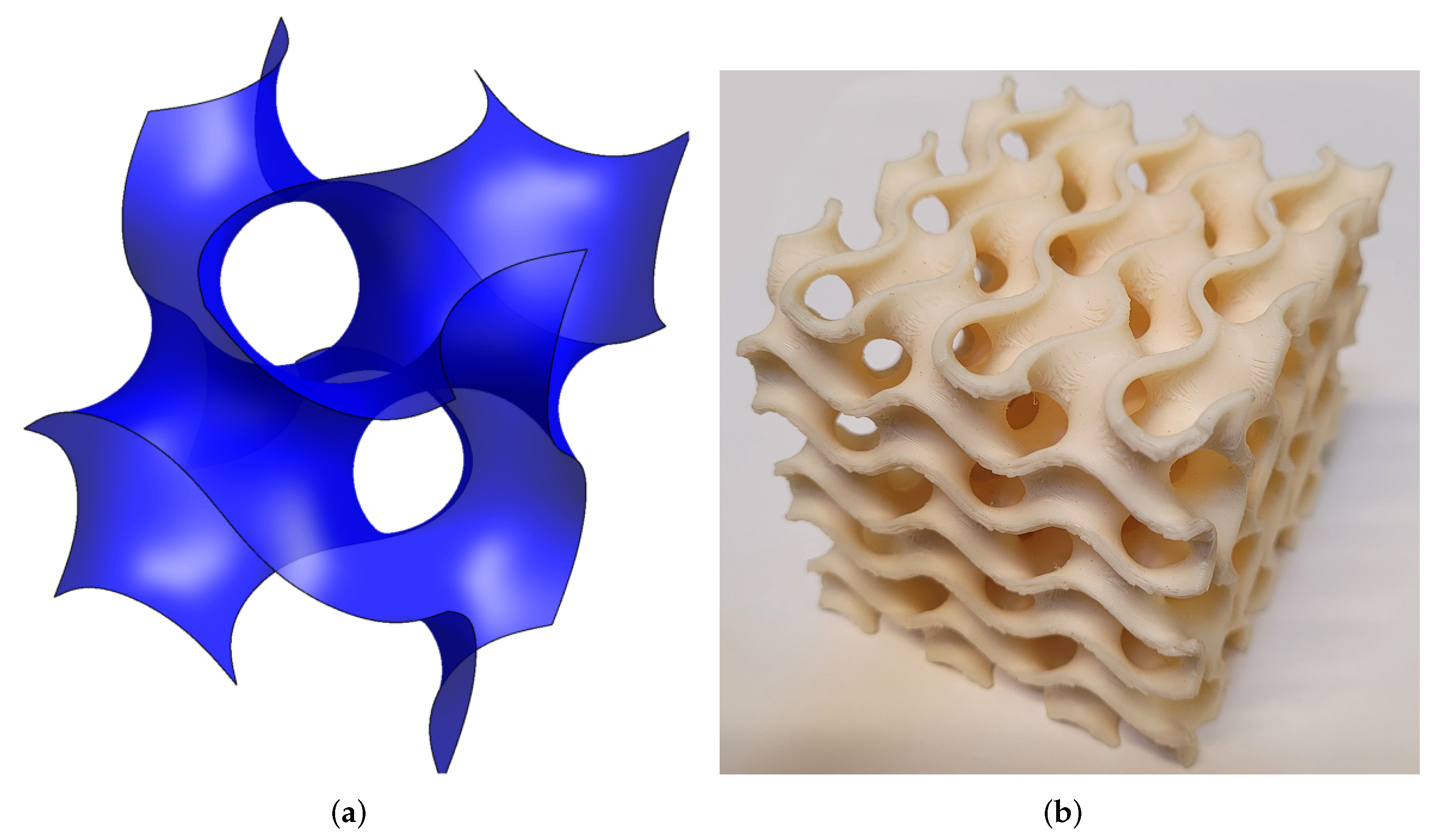
The gyroid surface ( see Figure 1) is one member in the mathematical family known as “triply-periodic minimal surfaces”, and was first discovered by Schoen [37] in 1970. The gyroid is defined by an implicit trigonometric Equation (1).
Upon its recent addition as an infill option in some slicers, the gyroid has produced much interest among hobbyist printers due to its beneficial properties such as near isotropy, quick print time, and strength [13,14,15]. For this research, the gyroid has been selected as the primary focus, and will be analyzed using the finite element method in order to develop predictive models of its behavior as the relative density varies, while the focus of this work is on the gyroid, the same method will be useful as additional 3D infills are implemented. In particular, infills with complex-shapes (such as other triply-periodic minimal surfaces) may warrant detailed investigation.
It is important to note that there are two types of gyroid infill. The first, which is the focus of this work, is that defined by thickening the gyroid minimal surface. The second is a separate but related infill that has been investigated by Zhang et al. [38] and others. Rather than a thickened minimal surface, this second type is a lattice of intersecting curved struts defined by filling in the empty space that the gyroid surface encloses. This “gyroid-strut” model has great potential regarding continuously variable relative density [38], however, it has not yet been implemented in common slicers.
In order to determine the elastic response of the gyroid infill, finite element analysis (FEA) was implemented to model a unit cell, similar to that done by Bhandari and Lopez-Anido [10,11,12]. Unlike the rectangular infill, however, the gyroid is a complexly curved surface and cannot be reasonably simplified to a space-frame model. The logical first step in analyzing this shape, then, was to use a shell model.
2.2. Shell Element Discretization
In a shell model, the midsurface of the part is represented by a series of thin elements. The formulation is based on the plane stress assumption wherein the only significant stress components are the in-plane normal and shear stresses due to bending moments and in-plane forces. The out-of-plane normal and shear stresses are typically small for a thin shell element and can be neglected. For the purpose of modeling the gyroid, it was assumed that, for low relative densities, these through-thickness effects are small enough as to be insignificant.
The first step in modeling the gyroid is to generate a mesh of the surface using triangular shell elements. Since tools for generating such a mesh based on an implicit equation were not readily available, this needed to be done using a purpose-built script, which built up the mesh using implicit function plotting tools to locate nodes along the surface. These nodes were then triangulated into a mesh. Since the implicit plotting tools are optimized for properly displaying the geometry rather than for numerical analysis, the resulting mesh contained a number of elements whose shapes were unacceptable for FEA modeling. To remedy this, a series of mesh cleanup steps were performed using mesh-smoothing, and remeshing tools included in an FEA software. These cleanup tools rearrange nodes within the surface with minimal out-of-plane deviation in order to produce a mesh which matches the geometry, but whose elements are closer to the ideal equilateral triangles for FEA. The final mesh can be seen in Figure 2. The meshed gyroid was then analyzed using FEA with periodic boundary conditions (discussed in Section 2.4), and assuming a linear elastic response. Due to the nature of the periodic boundary conditions, each node on a boundary of the RVE must correspond exactly with one node on the opposite boundary. This adjustment is made by re-seeding the boundaries with nodes that correspond with each other, and re-aligning the mesh to these new bounding-nodes.
In order to simulate different relative densities, several different shell thicknesses were modeled, and a curve of stiffness vs. relative density was generated. These showed clear deviation from expected behavior, particularly at high relative densities where the gyroid is expected to approach neat-material behavior. At these high relative densities, the structure is no longer thin-walled, which means that the shell assumptions are invalid and through-thickness stress effects are not negligible. Additionally, in some cases the thickness in the shell creates material overlap, thus double counting certain regions.
2.3. Solid Element Discretization
In order to ameliorate the shell issues and accurately predict the high relative density gyroid’s behavior, a solid-model was developed.
To generate this model, the shell midsurface was converted to a solid model by first taking a 3 × 3 × 3 unit-cell shell mesh as an .stl file, and thickening it by offsetting it along the normal. This geometry is then trimmed down to a single unit-cell to remove the edge distortion caused by the offsetting tool. The result was an .stl of the outer surface of the thickened gyroid. This mesh is cleaned up using the same remeshing tools as the shell model, and the boundary nodes adjusted for compatibility with the periodic boundary constraints. Here, the boundary adjustment was accomplished by completely replacing a boundary face with the mesh from the opposite face. Finally, the thickened surface mesh was converted to a solid using an automatic tetramesher which builds a mesh of solid tetrahedral elements to fill the space enclosed by the triangular surface mesh. The resulting solid model (see Figure 3) was analyzed using the same process as the shell model (linear response under periodic boundary conditions). In addition, a mesh convergence study was performed, the results of which can be found in Section 4.
2.4. Periodic Boundary Conditions and Elastic Property Calculations
Periodic boundary conditions allow for the modeling of a bulk material using a representative volume element (RVE). In order to do this, the nodes on the boundary of the RVE are constrained so that each boundary node’s displacements are matched to those of the corresponding node on the opposite boundary. An RVE constrained in this way has been shown to deform as if it were a single member in a bulk material composed of identical RVEs repeating in all directions [39]. The requirement that nodes be matched with corresponding nodes on opposite faces adds one additional step to the mesh generation, wherein the boundaries are re-seeded with nodes that correspond with each other, and the mesh realigned to these new bounding-nodes.
Once the boundary constraints are in place, a displacement is applied to one face, with the remaining faces free of traction. The resulting forces and displacements of the nodes are then calculated using FEA. Sun and Vaidya [39] demonstrated using Gauss’ divergence theorem that the average strain through the RVE can be determined directly from the displacement of the surface (2),
where V is RVE volume, S is a boundary surface, is displacement in the i-direction, is the i-component of the surface normal, and is the averaged component of the strain tensor. (3) shows how this reduces to the conventional strain definition for longitudinal strains in the x-direction,
where is the average normal component of strain in the x-direction, and are the length and elongation in the x-direction, respectively.
Likewise, using the principle of strain energy and external work equivalence, the average stress is shown to be by the applied force divided by the area of the surface [39] (4),
where is the average normal component of stress in the x-direction, is the normal force resultant summed across the boundary () of the RVE, and is the area of this face.
While the local stresses and strains vary throughout the model, these “average” properties are the behavior observed in a bulk material composed of these RVEs. The applied strain and predicted stress can then be used to calculate the effective elastic properties of this bulk-structure. Several similar analyses are needed to determine all of the properties of the bulk structure in different directions. Normal strains applied in any of the cardinal directions allow for calculation of the corresponding longitudinal modulus and the two corresponding Poisson’s ratios. For example, applying a normal displacement to the boundary () of the RVE causes it to deform such that there is also a length change in the y, and z-directions ( and ), and nodal resultant forces along the face which sum to . Dividing by the area of the face yields a resultant stress. These deformations/resultants are used in the standard definition of elastic modulus and Poisson’s ratio (5)–(7).
Likewise, to calculate shear modulus , a pure-shear state is imposed on the RVE by displacing the face in the y-direction by an amount , and the face face in the x-direction by an amount . This generates resultant shear forces on these faces ( and , respectively). As before, these deformations and resultants are used in the standard formula for shear modulus (8). Figure 4 demonstrates the deformation in these two cases.
For convenience, the constraints were generated, and requisite analyses were performed using an Abaqus plugin developed by Omairey et al. [40]. This results in 12 separate properties for the gyroid, however, there is little difference in the longitudinal moduli (, , and ), or the shear moduli (, , and ), or Poisson’s ratios (, , , , , and ). The gyroid exhibits cubic symmetry, meaning that the elastic behavior is fully defined using three independent constants: E, , and G. Any difference between the different directional properties arises from mesh imperfection. For this reason, the several properties are averaged to one constant each (see (9)–(11)).
Figure 5 shows the deformation of a representative gyroid solid model under the different loading modes. It is clear that the stress is not distributed uniformly through the structure, but rather concentrates in certain locations. The bulk elastic properties, however, are calculated from the average stresses and strains of the entire RVE.
3. Compression Experiments
In order to validate the FEA predictions, a series of compression experiments were conducted. The samples tested are prismatic rectangular blocks 152.4 mm × 50.8 mm × 50.8 mm () printed of Ultimaker toughened PLA on an Ultimaker 5 machine using a 0.4 mm nozzle with layer height 0.2 mm, extruder-temperature 205 C, bed-temperature 60 C, and print-speed 70 mm/s. Density was adjusted using the “Infill Density” and “Infill Line Multiplier” parameters in the Cura slicer. Wall thickness and top/bottom thickness parameters set to 0 to print bare infill. All other parameters remain default for an Ultimaker 5 machine. The size was chosen in order to capture the bulk behavior of the gyroid infill better than the standard compression specimen (which is much smaller) due to the printed unit-cell size. Cell-size and wall-thickness are the two driving factors for gyroid relative density. Since wall-thickness is fixed by the printer’s bead-width, the slicer adjusts relative density by changing the cell-size. The double-bead printed specimens at 25%, for example, are only 6 unit-cells wide. A smaller specimen would likely have significant edge-effects at this relative density. While the majority of these specimens are printed so that the testing direction corresponded with the z-axis of the printer, others are printed in the x-, and y-directions, respectively, in order to capture any directional effects. These specimens are labeled separately in the results. All of the specimens were tested using an Instron 100 kN servohydraulic test frame in quasi-static compression. Compression was chosen so as to capture longitudinal stresses while avoiding potential issues with gripping a porous structure. This test was based on ASTM D695 [44], but with the aforementioned deviation in specimen size. These experiments are displacement-controlled with a feed rate of 1.27 mm/min (0.05 in/min). In addition, any extraneous moments due to fixture misalignment are eliminated by using a swiveling top platen (see Figure 6).
Load data is captured using a 100 kN load cell and strain data is captured using digital image correlation (DIC). DIC data is captured in the form of a pointwise displacement field based on a series of dots adhered to the surface of each specimen. Analyzing this data using the GOM Correlate software, a surface is generated wherein the dots become the corner nodes of a mesh. The longitudinal and transverse strains are then calculated at each node using the built-in analysis tools. It is noteworthy that neither longitudinal nor transverse strain vary noticeably across the measured region (Figure 7 demonstrates how little the transverse strain varies), which indicates that the gauge region is sufficiently distant from the testing fixtures as to be outside the edge-effected area.
This test was performed with several specimens each at 25%, 50%, 75%, and 100% nominal relative density. For each relative density (except 100%) two different geometries are used: one-bead and two-bead wall thicknesses. This is in order to determine whether the wall-thicknesses are a significant factor in the response. Nominal density of each specimen is defined as a parameter in the slicing software, while the actual density is determined by measuring its size and mass. This is then divided by the published density of PLA to convert to relative density.
4. Results and Discussion
4.1. Mesh Convergence
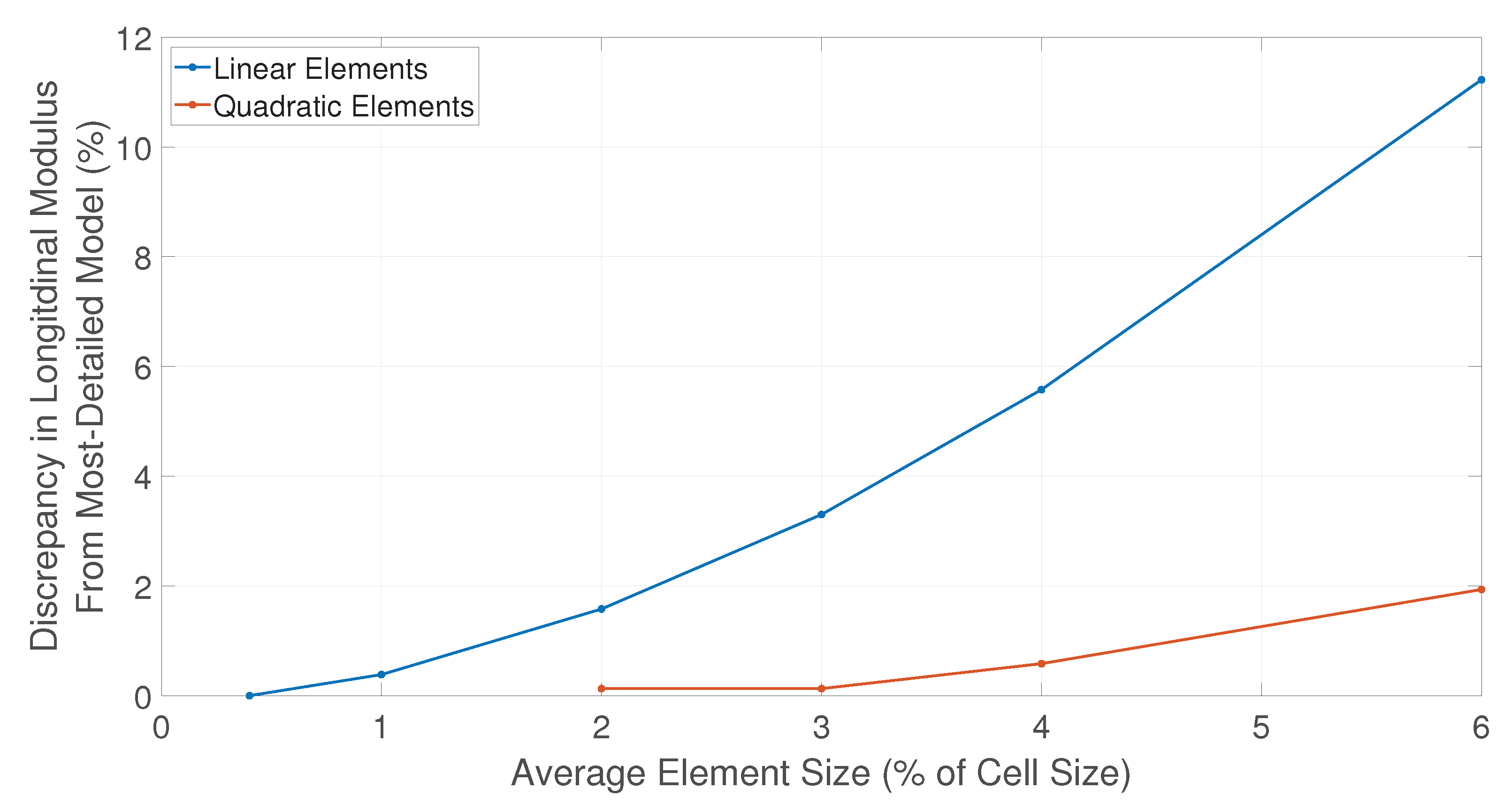
In order to guarantee that mesh-size effects are not significant in the final results, a convergence study has been performed using the 50% relative density 3D model. Based on the results of this study (Figure 8), all subsequent analyses were performed using 10-noded quadratic tetrahedral elements. These elements have an average size that is 2% of the cell size. Average size is specified here because the models for different relative densities all have different numbers of elements, but the average size remains constant in all of the models.
4.2. Shell vs. Solid Models
In this section, the results obtained from the shell model are compared with those obtained from the solid model. Figure 9 shows that the shell model matches the solid for the lower relative density portion of the plot, but the two models rapidly diverge above 40% relative density. At these higher relative densities, the solid model more accurately matches the expected result by approaching 100% of the neat stiffness as it approaches 100% relative density. As such, the solid model results have been used for all comparisons to experimental data and for curve fitting. This additional accuracy does come at the cost of increased complexity, and computation time. In addition, to simulate different relative densities using solid models requires that the thickening process be performed to generate a new mesh for each relative density to be analyzed, where the shell-model’s relative density can be adjusted by simply altering the shell-thickness parameter. For these reasons, it would be best to use shell models in any instance where their accuracy is sufficient such as on the low end of the relative density range.
4.3. Compression Results
Stress–strain curves are shown in Figure 10. These samples are clearly seen to exhibit elastic–plastic behavior similar to those samples of ULTEM 9085 tested by Bhandari and Lopez-Anido [12]. Based on qualitative observation of the many simulation results, this failure seems to be a combination of the local elastic instability/buckling and plastic failure. As a bulk property, however, this can be captured simply as an elastic-plastic response.
Table 1 shows a summary of results from the compression tests. From this data, we can see that the actual measured relative densities of 2-bead thickness specimens are much closer to the nominal relative density, especially for higher relative densities. For example, the single-bead 75% infill specimens are actually closer to 50% relative density, whereas the double-bead variant is exactly the nominal 75% relative density. For this reason, it is assumed that the printer cannot properly resolve the gyroid geometry using a single-bead. It is important to note that the relative density of the gyroid is determined by two factors: the unit-cell size, and the wall thickness. Since wall thickness is fixed here (by the bead-width of the print), the way in which relative density is altered is by varying unit-cell size. This means that of the specimens printed, the 75% single-bead specimens have the smallest cell size, which explains why the resolution issue is most pronounced in these specimens.
4.3.1. Longitudinal Modulus
Elastic modulus was determined for each of the specimens by fitting a line to the initial linear portion of the stress–strain response. Figure 11 shows a comparison between experimental data and predicted values. On this plot, it is clear that, while there is some variation from specimen to specimen, the experimental data agrees well with that predicted. Note that due to the variation in results, these data were normalized against a reference material properties drawn from the PLA filament manufacturer’s published modulus and density data (rather than against measured values from the 100% infill test-specimens). It is also worth noting that for both modulus and Poisson’s ratio, the z-orientation (default) specimens vary only slightly from their x- and y-orientation counterparts at 50% relative density.
4.3.2. Poisson’s Ratio
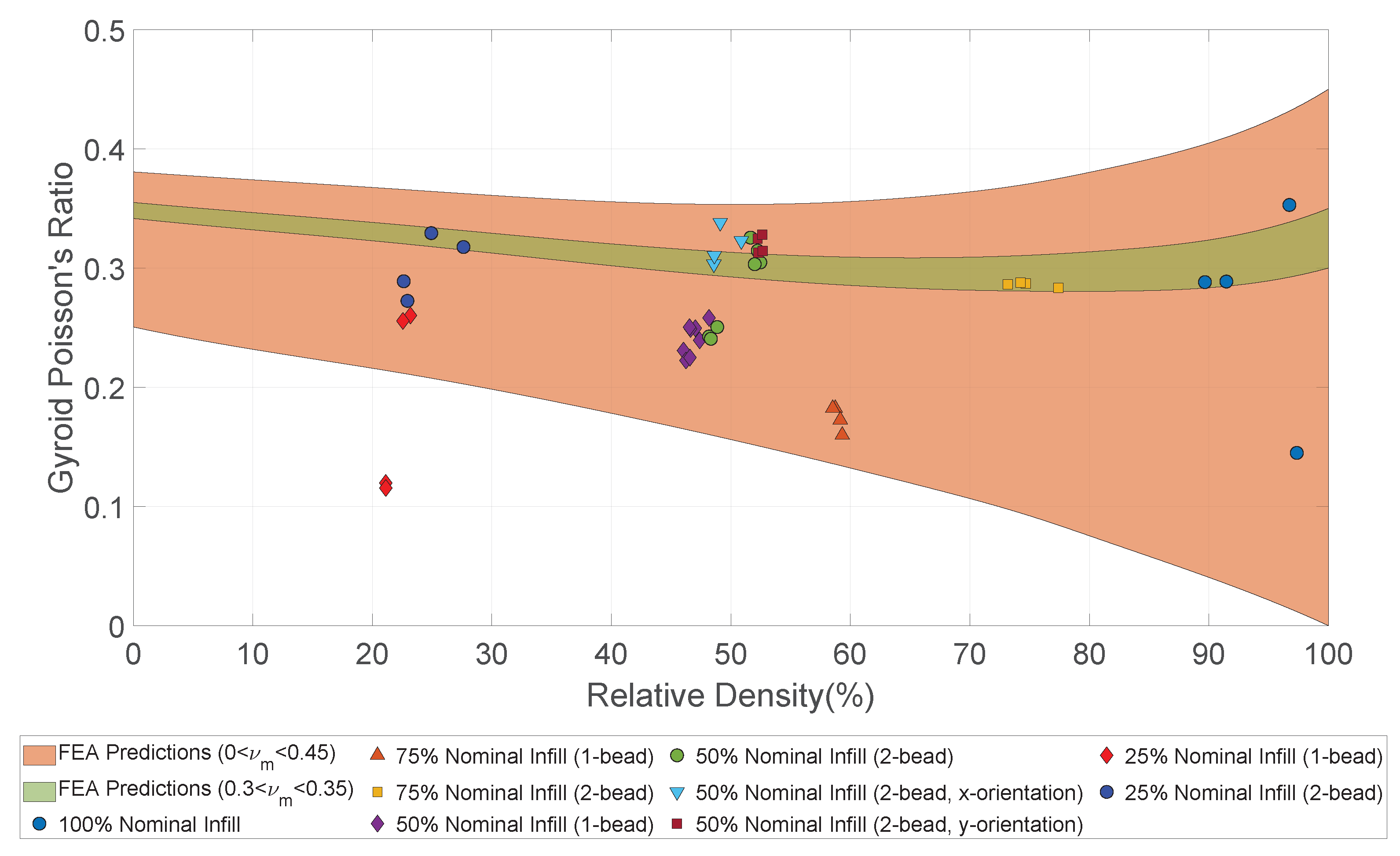
Poisson’s ratio of the test specimens was determined by first averaging the strains across the gauge region of the specimen, then taking the ratio of average transverse strain and average longitudinal strain. In order to minimize data noise and capture the overall behavior through the linear portion of the test, this was calculated using a linear regression for vs. . Figure 12 shows the measured Poisson’s ratio data points along with the FEA predicted ranges for the gyroid’s Poisson response. Since published data for the Poisson’s ratio of neat-PLA ranges from 0.3 to 0.35, it is anticipated that these gyroid specimens, being printed from PLA, should have a Poisson’s ratio that falls within the window. This data, however, shows a significant amount of scatter; enough that the variation between specimens is larger in some cases than the variation that was predicted for . In addition, it is clear that the double-bead thickness specimens match the FEA predictions much better than do the single-bead specimens. This, in addition to the issue with matching desired relative density, indicates that it is best to use a double-bead infill for structural predictability.
From this data, we can see that the modulus predictions match reality quite well, and the Poisson’s ratio predictions match for specimens with 2-bead wall thicknesses.
4.4. Semi-Empirical Models
In Section 2, a method was presented for generating predictive solid models of the gyroid infill. These solid-model analyses were performed several times at each of several relative densities over a range of test materials with modulus values () from 1000 to 4000 MPa, and Poisson’s ratio values () ranging from 0 to 0.45. (Since the base material is isotropic, the shear modulus is calculated from them using the standard isotropic relationship.) This range of properties was chosen to encompass the behavior of a variety of common 3D printing polymers, so as to allow for predictions with all of these materials. In order to best use the resulting predictions for design, a relatively simple equation is defined which fits the data. This is similar to how simple mathematical models have been used to predict the behavior of other cellular structures such as honeycombs or foams [45].
4.4.1. Longitudinal Modulus
The starting point for this effort is to find a model that properly predicts the longitudinal modulus of the gyroid at various relative densities. By looking at a plot of the FEA results, it is clear that the gyroid’s longitudinal modulus (), when normalized against the neat material modulus (), is nearly independent of all parameters except relative density. A variety of models have been found in the literature relating to cellular structures such as foams and honeycombs. For example, a power law is used to represent the modulus of closed-cell foams in [46]. In addition, a variety of polynomial ratios have been used for various foam and honeycomb predictions in [47,48,49,50,51]. None of these, however, fit the data satisfactorily. The model found to best fit the data was a modified power law,
where is the normalized longitudinal modulus, is the neat-material elastic modulus, are curve fitting coefficients, and D is the relative density of infill ( which corresponds to ). The best value of fitting parameters and were determined to be 0.77 and 1.2, respectively. This results in an average error of 0.44% (maximum 1.13%). Figure 13 shows the FEA and semi-emperical predictions.
4.4.2. Shear Modulus
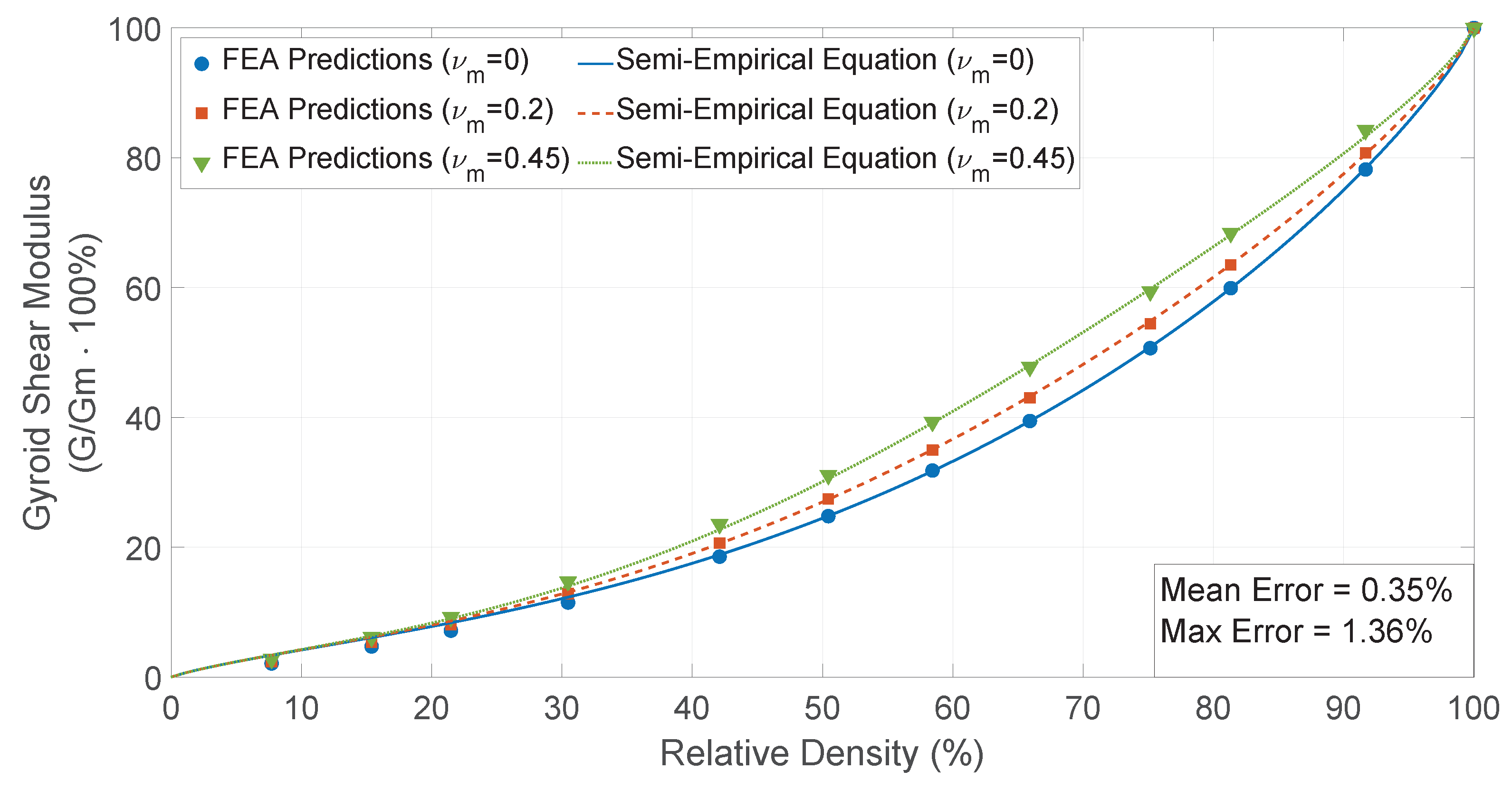
While shear modulus has not yet been verified experimentally, it was calculated in the FEA analysis so the results have also been curve fit for simplicity of use. Unlike the longitudinal modulus, the normalized shear modulus is seen to be a function of both relative density and Poisson’s ratio. As such, very few different types of model have been found in cellular structures or composites literature which are applicable. Gong et al. [50] and Ghezal et al. [48] predict different responses for shear response, but neither of these results in a satisfactory fit for the gyroid. Likewise, simple modifications of the basic mathematical models yield unsatisfactory results. It is apparent, however, that the normalized shear modulus follows a similar curve to the longitudinal modulus. In fact, simply using the curve results in a max error of only 9.3%. This is improved significantly with the addition of a Poisson’s ratio dependent term, yielding (13). The form of this term was determined by curve fitting various functional forms and choosing the one which resulted in the smallest error.
where is the normalized shear modulus, is the neat-material shear modulus, and is the neat-material Poisson’s ratio. The best value of fitting parameter was determined to be 0.5. This results in an average error of 0.35% (maximum 1.36%). Figure 14 shows the FEA and semi-emperical predictions.
4.4.3. Poisson’s Ratio
Similar to the shear modulus, there are very few models in the literature to predict the bulk Poisson’s ratio of cellular microstructures. By removing the purely geometric component of the response (Poisson’s ratio resulting from a gyroid of zero-Poisson material), it was found that this also follows a similar curve to the longitudinal modulus. Figure 15 shows the FEA and semi-emperical predictions.
where the geometric component is represented by the polynomial:
The best value of fitting parameters , , and were determined to be 0.28, 0.088, and 0.16, respectively. This produces an average error of 1.59% (maximum 6.54%).
4.5. Degree of Anisotropy
A common metric for determining the anisotropy of a material with cubic symmetry is the Zener index [52] (or Zener ratio), which is defined by (16).
Isotropic materials have Zener index of one. The further from one, the more anisotropic the material. The Zener index has been calculated for the gyroid using the semi-empirical equations developed previously, and the results plotted in Figure 16.
The figure shows that the gyroid’s Zener index varies with varying density, but that it remains close to one (). By comparison, some other cubically symmetric infills have been shown to exhibit Zener ratios above two [53]. It is clear, then, that the gyroid is very-nearly isotropic. This near isotropy greatly simplifies implementation of gyroids into design and optimization workflows.
5. Conclusions
A novel homogenization method has been developed whereby FEA can be utilized to determine effective elastic properties of 3D printed infills. By discretizing the infill’s unit cell and applying periodic boundaries, a prediction of the bulk elastic properties is made for a given relative density.
This method has been applied to the gyroid infill by performing a full suite of simulations. This allowed for generation of predictive data for the effective elastic properties at the full range of relative densities, using various base-materials. The FEA predictions have been verified using compression experiments whose results correspond well to the predicted behavior. At 50% nominal density, the error in longitudinal modulus is only 4% of neat modulus, which is less than the variation within the test results (5%). Finally, the FEA predictions have been used in order to inform semi-empirical equations, which can be used directly in designing parts using gyroid infill. These equations match the FEA predictions do a high degree of accuracy (0.44% error for the longitudinal modulus).
It is clear that a method of predicting homogeneous bulk properties of infills is an important component in optimal design using AM technology. The method presented here will likely be very useful in designing components using any of the complex 3D infills.
Author Contributions
The following is a list of the contributions by the various authors: Conceptualization, R.A.L.-A., S.V. and P.B.; methodology, P.B.; software, P.B.; formal analysis, P.B.; investigation, P.B.; resources, R.A.L.-A. and S.V.; data curation, P.B.; writing—original draft preparation, P.B.; writing—review and editing, R.A.L.-A., S.V. and P.B.; visualization, P.B.; supervision, R.A.L.-A. and S.V.; project administration, R.A.L.-A. and S.V.; funding acquisition, R.A.L.-A. All authors have read and agreed to the published version of the manuscript.
Funding
This research was funded under the U.S. Army Natick Soldier Systems Center, and has been approved for public release—DEVCOM SC PR2021-30271.
Institutional Review Board Statement
Not applicable.
Informed Consent Statement
Not applicable.
Data Availability Statement
Not applicable.
Acknowledgments
This research was done in partnership with the University of Maine Advanced Structures and Composites Center. Special thanks to the Scott Tomlinson, Paul Bussiere, and the Additive Manufacturing Team!
Conflicts of Interest
The authors declare no conflict of interest.
Abbreviations
The following abbreviations are used in this manuscript:
| AM | Additive Manufacturing |
| FEA | Finite Element Analysis |
| RVE | Representative Volume Element |
| DIC | Digital Image Correlation |
References
- Jiang, J.; Fu, Y.F. A short survey of sustainable material extrusion additive manufacturing. Aust. J. Mech. Eng. 2020, 1–10. [Google Scholar] [CrossRef]
- Jiang, J.; Ma, Y. Path Planning Strategies to Optimize Accuracy, Quality, Build Time and Material Use in Additive Manufacturing: A Review. Micromachines 2020, 11, 633. [Google Scholar] [CrossRef]
- Lee, H.; Lim, C.H.J.; Low, M.J.; Tham, N.; Murukeshan, V.M.; Kim, Y.J. Lasers in additive manufacturing: A review. Int. J. Precis. Eng. Manuf. Green Technol. 2017, 4, 307–322. [Google Scholar] [CrossRef]
- Fu, Y.F.; Rolfe, B.; Chiu, L.N.; Wang, Y.; Huang, X.; Ghabraie, K. Parametric studies and manufacturability experiments on smooth self-supporting topologies. Virtual Phys. Prototyp. 2020, 15, 22–34. [Google Scholar] [CrossRef]
- Bikas, H.; Stavropoulos, P.; Chryssolouris, G. Additive manufacturing methods and modelling approaches: A critical review. Int. J. Adv. Manuf. Technol. 2016, 83, 389–405. [Google Scholar] [CrossRef] [Green Version]
- Khorasani, M.; Ghasemi, A.; Rolfe, B.; Gibson, I. Additive manufacturing a powerful tool for the aerospace industry. Rapid Prototyp. J. 2021, 28, 87–100. [Google Scholar] [CrossRef]
- Tan, C.; Zou, J.; Li, S.; Jamshidi, P.; Abena, A.; Forsey, A.; Moat, R.J.; Essa, K.; Wang, M.; Zhou, K.; et al. Additive manufacturing of bio-inspired multi-scale hierarchically strengthened lattice structures. Int. J. Mach. Tools Manuf. 2021, 167, 103764. [Google Scholar] [CrossRef]
- Kumar, M.; Sharma, V. Additive manufacturing techniques for the fabrication of tissue engineering scaffolds: A review. Rapid Prototyp. J. 2021, 27, 1230–1272. [Google Scholar] [CrossRef]
- Gibson, I.; Rosen, D.W.; Stucker, B.; Khorasani, M. Additive Manufacturing Technologies; Springer: Cham, Switzerland, 2021; Volume 17. [Google Scholar]
- Bhandari, S. Feasibility of Using 3D Printed Molds for Thermoforming Thermoplastic Composites. Master’s Thesis, University of Maine, Orono, ME, USA, 2016. [Google Scholar]
- Bhandari, S.; Lopez-Anido, R. Finite element modeling of 3D-printed part with cellular internal structure using homogenized properties. Prog. Addit. Manuf. 2019, 4, 143–154. [Google Scholar] [CrossRef]
- Bhandari, S.; Lopez-Anido, R. Finite element analysis of thermoplastic polymer extrusion 3D printed material for mechanical property prediction. Addit. Manuf. 2018, 22, 187–196. [Google Scholar] [CrossRef]
- 3D Metal Forge. Gyroid Infills for 3D Printing. Available online: https://3dmetalforge.com/en/gyroid-infills-for-3d-printing-2/ (accessed on 6 February 2020).
- Goldschmidt, B. The Best Cura Infill Pattern (For Your Needs). Available online: https://all3dp.com/2/cura-infill-patterns-all-you-need-to-know/ (accessed on 6 February 2020).
- Matt’s Hub. Introducing Gyroid Infill. Available online: https://mattshub.com/blog/2018/03/15/gyroid-infill (accessed on 6 February 2020).
- Li, D.; Dai, N.; Jiang, X.; Chen, X. Interior structural optimization based on the density-variable shape modeling of 3D printed objects. Int. J. Adv. Manuf. Technol. 2016, 83, 1627–1635. [Google Scholar] [CrossRef]
- Sundararajan, V.G. Topology Optimization for Additive Manufacturing of Customized Meso-Structures Using Homogenization and Parametric Smoothing Functions. Ph.D. Thesis, University of Texas at Austin, Austin, TX, USA, 2010. [Google Scholar]
- Xie, Y.; Chen, X. Support-free interior carving for 3D printing. Vis. Inform. 2017, 1, 9–15. [Google Scholar] [CrossRef]
- Lu, L.; Chen, B.; Sharf, A.; Zhao, H.; Wei, Y.; Fan, Q.; Chen, X.; Savoye, Y.; Tu, C.; Cohen-Or, D. Build-to-last: Strength to Weight 3D Printed Objects. ACM Trans. Graph. 2014, 33, 1–10. [Google Scholar] [CrossRef]
- Clausen, A.; Aage, N.; Sigmund, O. Topology optimization of coated structures and material interface problems. Comput. Methods Appl. Mech. Eng. 2015, 290, 524–541. [Google Scholar] [CrossRef] [Green Version]
- Gaynor, A.T.; Meisel, N.A.; Williams, C.B.; Guest, J.K. Multiple-Material Topology Optimization of Compliant Mechanisms Created Via PolyJet Three-Dimensional Printing. J. Manuf. Sci. Eng. 2014, 136, 061015. [Google Scholar] [CrossRef] [Green Version]
- Riss, F.; Schilp, J.; Reinhart, G. Load-dependent optimization of honeycombs for sandwich components-new possibilities by using additive layer manufacturing. Phys. Procedia 2014, 56, 327–335. [Google Scholar] [CrossRef]
- Chu, J.; Engelbrecht, S.; Graf, G.; Rosen, D.W. A comparison of synthesis methods for cellular structures with application to additive manufacturing. Rapid Prototyp. J. 2010, 16, 275–283. [Google Scholar] [CrossRef] [Green Version]
- Schumacher, C.; Bickel, B.; Rys, J.; Marschner, S.; Daraio, C.; Gross, M. Microstructures to control elasticity in 3D printing. ACM Trans. Graph. 2015, 34, 1–13. [Google Scholar] [CrossRef] [Green Version]
- Wu, J.; Wang, C.C.; Zhang, X.; Westermann, R. Self-supporting rhombic infill structures for additive manufacturing. Comput. Aided Des. 2016, 80, 32–42. [Google Scholar] [CrossRef]
- Brackett, D.; Ashcroft, I.; Hague, R. Topology optimization for additive manufacturing. Solid Free. Fabr. Symp. 2011. [Google Scholar] [CrossRef]
- McCaw, J.C.; Cuan-Urquizo, E. Mechanical characterization of 3D printed, non-planar lattice structures under quasi-static cyclic loading. Rapid Prototyp. J. 2020, 26, 707–717. [Google Scholar] [CrossRef]
- Tsouknidas, A.; Pantazopoulos, M.; Katsoulis, I.; Fasnakis, D.; Maropoulos, S.; Michailidis, N. Impact absorption capacity of 3D-printed components fabricated by fused deposition modelling. Mater. Des. 2016, 102, 41–44. [Google Scholar] [CrossRef]
- Lužanin, O.; Movrin, D.; Plan, M. Effect of Layer Thickness, Deposition Angle, and Infill on Maximum Flexural Force in Fdm-Built Specimens. J. Technol. Plast. 2014, 39, 49–58. [Google Scholar]
- Baich, L.; Manogharan, G.; Marie, H. Study of infill print design on production cost-time of 3D printed ABS parts. Int. J. Rapid Manuf. 2015, 5, 308–319. [Google Scholar] [CrossRef]
- Wang, W.; Wang, T.Y.; Yang, Z.; Liu, L.; Tong, X.; Tong, W.; Deng, J.; Chen, F.; Liu, X. Cost-effective printing of 3D objects with skin-frame structures. ACM Trans. Graph. 2013, 32, 1–10. [Google Scholar] [CrossRef] [Green Version]
- Marschall, D.; Sindinger, S.L.; Rippl, H.; Bartosova, M.; Schagerl, M. Design, simulation, testing and application of laser-sintered conformal lattice structures on component level. Rapid Prototyp. J. 2021, 27, 43–57. [Google Scholar] [CrossRef]
- Shaikh, M.Q.; Graziosi, S.; Atre, S.V. Supportless printing of lattice structures by metal fused filament fabrication (MF3) of Ti-6Al-4V: Design and analysis. Rapid Prototyp. J. 2021, 27, 1408–1422. [Google Scholar] [CrossRef]
- Li, D.; Qin, R.; Chen, B.; Zhou, J. Analysis of mechanical properties of lattice structures with stochastic geometric defects in additive manufacturing. Mater. Sci. Eng. A 2021, 822, 141666. [Google Scholar] [CrossRef]
- Chan, Y.C.; Shintani, K.; Chen, W. Robust topology optimization of multi-material lattice structures under material and load uncertainties. Front. Mech. Eng. 2019, 14, 141–152. [Google Scholar] [CrossRef] [Green Version]
- Martínez, J.; Song, H.; Dumas, J.; Lefebvre, S. Orthotropic k-nearest foams for additive manufacturing. ACM Trans. Graph. 2017, 36, 1–12. [Google Scholar] [CrossRef] [Green Version]
- Schoen, A.H. Infinite Periodic Minimal Surfaces without Self-Intersections; Technical Report; NASA: Washington, DC, USA, 1970. [Google Scholar]
- Zhang, B.; Mhapsekar, K.; Anand, S. Design of Variable-Density Structures for Additive Manufacturing Using Gyroid Lattices. In Proceedings of the International Design Engineering Technical Conferences and Computers and Information in Engineering Conference, Cleveland, OH, USA, 6–9 August 2017; Volume 4. [Google Scholar]
- Sun, C.T.; Vaidya, R.S. Prediction of composite properties from a representative volume element. Compos. Sci. Technol. 1996, 56, 171–179. [Google Scholar] [CrossRef]
- Omairey, S.L.; Dunning, P.D.; Sriramula, S. Development of an ABAQUS plugin tool for periodic RVE homogenisation. Eng. Comput. 2019, 35, 567–577. [Google Scholar] [CrossRef] [Green Version]
- Theerakittayakorn, K.; Nanakorn, P. Periodic boundary conditions for unit cells of periodic cellular solids in the determination of effective properties using beam elements. In Proceedings of the 2013 World Congress on Advances in Structural Engineering and Mechanics (ASEM13), Jeju, Korea, 8–12 September 2013; pp. 3738–3748. [Google Scholar]
- Wu, W.; Owino, J.; Al-Ostaz, A.; Cai, L. Applying periodic boundary conditions in finite element analysis. In Proceedings of the SIMULIA Community Conference, Providence, Providence, RI, USA, 19–22 May 2014; pp. 707–719. [Google Scholar]
- Tyrus, J.; Gosz, M.; DeSantiago, E. A local finite element implementation for imposing periodic boundary conditions on composite micromechanical models. Int. J. Solids Struct. 2007, 44, 2972–2989. [Google Scholar] [CrossRef] [Green Version]
- ASTM D695-15; Standard Test Method for Compressive Properties of Rigid Plastics. American Society for Testing and Materials: West Conshohocken, PA, USA, 2015.
- Gibson, L.J.; Ashby, M.F. Cellular Solids: Structure and Properties, 2nd ed.; Cambridge University Press: Cambridge, MA, USA, 1997. [Google Scholar]
- Redenbach, C.; Shklyar, I.; Andrä, H. Laguerre tessellations for elastic stiffness simulations of closed foams with strongly varying cell sizes. Int. J. Eng. Sci. 2012, 50, 70–78. [Google Scholar] [CrossRef]
- Gibson, I.; Ashby, M.F. The mechanics of three-dimensional cellular materials. Proc. R. Soc. Lond. A Math. Phys. Sci. 1982, 382, 43–59. [Google Scholar]
- El Ghezal, M.I.; Maalej, Y.; Doghri, I. Micromechanical models for porous and cellular materials in linear elasticity and viscoelasticity. Comput. Mater. Sci. 2013, 70, 51–70. [Google Scholar] [CrossRef]
- Gibson, L. Modelling the mechanical behavior of cellular materials. Mater. Sci. Eng. A 1989, 110, 1–36. [Google Scholar] [CrossRef]
- Gong, L.; Kyriakides, S.; Jang, W.Y. Compressive response of open-cell foams. Part I: Morphology and elastic properties. Int. J. Solids Struct. 2005, 42, 1355–1379. [Google Scholar] [CrossRef]
- Ahmadi, S.; Campoli, G.; Yavari, S.A.; Sajadi, B.; Wauthlé, R.; Schrooten, J.; Weinans, H.; Zadpoor, A. Mechanical behavior of regular open-cell porous biomaterials made of diamond lattice unit cells. J. Mech. Behav. Biomed. Mater. 2014, 34, 106–115. [Google Scholar] [CrossRef]
- Zener, C. Elasticity and Anelasticity of Metals; University of Chicago Press: Chicago, IL, USA, 1948. [Google Scholar]
- Chen, Z.; Xie, Y.M.; Wu, X.; Wang, Z.; Li, Q.; Zhou, S. On hybrid cellular materials based on triply periodic minimal surfaces with extreme mechanical properties. Mater. Des. 2019, 183, 108109. [Google Scholar] [CrossRef]
Figure 1.
Examples of the gyroid geometry. (a) A 3D rendering of the gyroid minimal surface; (b) 3D printed gyroid.
Figure 1.
Examples of the gyroid geometry. (a) A 3D rendering of the gyroid minimal surface; (b) 3D printed gyroid.

Figure 2.
Example of a shell model of the gyroid structure unit-cell.

Figure 3.
Example of a solid model of the gyroid structure unit-cell (50% relative density).

Figure 4.
Examples deformations of the gyroid representative volume element (RVE) (adapted from [40]). (a) RVE with applied longitudinal strain; (b) RVE with applied shear strain.
Figure 4.
Examples deformations of the gyroid representative volume element (RVE) (adapted from [40]). (a) RVE with applied longitudinal strain; (b) RVE with applied shear strain.

Figure 5.
Deformed shape and stress distribution of a gyroid solid model (50% relative density). (a) Longitudinal deformation and stress (); (b) shear deformation and stress ().
Figure 5.
Deformed shape and stress distribution of a gyroid solid model (50% relative density). (a) Longitudinal deformation and stress (); (b) shear deformation and stress ().

Figure 6.
Gyroid prismatic specimen in the compression fixture.

Figure 7.
Digital image correlation (DIC) generated transverse-strain field (overlaying the capture image).
Figure 7.
Digital image correlation (DIC) generated transverse-strain field (overlaying the capture image).

Figure 8.
Mesh convergence data.

Figure 9.
Comparison of the normalized elastic moduli from the shell and solid models.

Figure 10.
Longitudinal stress–strain curves from the compression experiments.

Figure 11.
Experimental results vs. finite element analysis (FEA) predictions for elastic modulus.

Figure 12.
Experimental results vs. FEA predictions for Poisson’s ratio.

Figure 13.
FEA predictions vs. semi-empirical equation for longitudinal modulus.

Figure 14.
FEA predictions vs. semi-empirical equation for shear modulus.

Figure 15.
FEA predictions vs. semi-empirical equation for Poisson’s ratio.

Figure 16.
Zener index of gyroid infills.


Table 1.
Summary of experimental results.
| Nominal Relative Density | Wall Thicknesses | Avg Relative Density (%) | Londitudinal Modulus (MPa) | Poisson’s Ratio |
|---|---|---|---|---|
| 100% | - | 94 | 2300 | 0.25 |
| 75% | Single-Bead | 59 | 639 | 0.18 |
| 75% | Double-Bead | 75 | 1420 | 0.28 |
| 50% | Single-Bead | 47 | 490 | 0.24 |
| 50% | Double-Bead | 51 | 520 | 0.30 |
| 25% | Single-Bead | 22 | 145 | 0.19 |
| 25% | Double-Bead | 25 | 191 | 0.30 |
Publisher’s Note: MDPI stays neutral with regard to jurisdictional claims in published maps and institutional affiliations. |
© 2022 by the authors. Licensee MDPI, Basel, Switzerland. This article is an open access article distributed under the terms and conditions of the Creative Commons Attribution (CC BY) license (https://creativecommons.org/licenses/by/4.0/).
Share and Cite
MDPI and ACS Style
Bean, P.; Lopez-Anido, R.A.; Vel, S. Numerical Modeling and Experimental Investigation of Effective Elastic Properties of the 3D Printed Gyroid Infill. Appl. Sci. 2022, 12, 2180. https://doi.org/10.3390/app12042180
AMA Style
Bean P, Lopez-Anido RA, Vel S. Numerical Modeling and Experimental Investigation of Effective Elastic Properties of the 3D Printed Gyroid Infill. Applied Sciences. 2022; 12(4):2180. https://doi.org/10.3390/app12042180
Chicago/Turabian StyleBean, Philip, Roberto A. Lopez-Anido, and Senthil Vel. 2022. "Numerical Modeling and Experimental Investigation of Effective Elastic Properties of the 3D Printed Gyroid Infill" Applied Sciences 12, no. 4: 2180. https://doi.org/10.3390/app12042180
Note that from the first issue of 2016, this journal uses article numbers instead of page numbers. See further details here.