
Dynamic Structural Scaling Concept for a Delta Wing Wind Tunnel Configuration Using Additive Manufacturing
Chair of Aerodynamics and Fluid Mechanics, School of Engineering and Design, Technical University of Munich, 85748 Garching bei München, Germany
*
Author to whom correspondence should be addressed.
Aerospace 2023, 10(7), 581; https://doi.org/10.3390/aerospace10070581
Submission received: 2 May 2023
/
Revised: 7 June 2023
/
Accepted: 18 June 2023
/
Published: 22 June 2023
(This article belongs to the Special Issue Applied Aeroelasticity and Fluid-Structure Interaction)
Abstract
:Considering aeroelastic effects plays a vital role in the aircraft design process. The construction of elastic wind tunnel models is a critical element in the investigation of occurring aeroelastic phenomena. However, the structural scaling between full-scale and reduced-scale configurations is a complex design and manufacturing task and is usually avoided in wind tunnel testing. This work proposes a numerical approach for a dynamic aeroelastic scaling technique, which is applied to a fictive delta wing configuration. This scaling methodology is designed to optimise the structural layout of wind tunnel models with an integrated rib and spar structure to meet the behaviour of a realistic full-scale equivalent. For the modelling approach of the wing structure, a beam and shell structure is utilised. The applied scaling laws for the relevant quantities and the applied procedures are described. Computational fluid dynamics (CFD) calculations are performed by solving the Reynolds-averaged Navier–Stokes (RANS) equations for the assumption of a rigid full-scale and down-scaled wing. These calculations are used to verify the aerodynamic scaling assumptions, which are applied to the scaling procedure of the wind tunnel model. Global aerodynamic coefficients are evaluated for a variety of angles of attack. The local flow phenomena of the full-scale and the scaled model are compared in more detail for a medium and a high angle of attack. The pressure coefficient distribution shows a proper accordance for the full-scale and the scaled model. To verify the results of the structural scaling optimisation, a high-fidelity structural full-scale model is compared with the scaled model using the ELFINI FEM solver. Therefore, all structural components are modelled by 2D elements. The results for the reduced eigenfrequencies and according modes of the full-scale and the scaled model show a high level of similarity. A static deformation of the structural grids is performed by applying the aerodynamic loads from the CFD simulations. The results show that the deviation of the nondimensional deformation between the scaled and the full-scale model is negligible. Consequently, the applied scaling methodology proves to be a valuable tool for the conceptual approach of designing aeroelastically scaled wind tunnel models considering 3D-printed material.
1. Introduction
The investigation of highly agile delta-wing aerodynamics considering deformable mechanical structures plays an important role in aeronautical research. In this context, the elastic deformation of aircraft structures is considered for an applied aerodynamic loading. The occurring deformations retroactively influence the aerodynamic characteristics of the aircraft, leading to a complex coupling between the fluid and the structure of the aircraft. Despite the slender structure of delta wings, which feature small aspect ratios, elastic deformations play a major role. This is due to several factors. First, thin airfoils are used for the wing layout to meet the requirements for low drag in the supersonic regime of the flight envelope. The choice of thin airfoils favours considerable deformations. In addition, massive loads occur on the wings in the high angle-of-attack range, which contribute to large deformations even at moderate flow velocities.
In this work, a fictive delta wing configuration with a deployed slat is investigated for low-speed conditions at high angles of attack. For these conditions, the flow around high-agility aircraft configurations is characterised by complex phenomena that have been investigated in detail in the last decades [1,2]. In general, the flow around highly swept wing configurations with a low to medium aspect ratio is determined by the formation of complex vortex systems and areas of strongly separated flow. These phenomena occur for medium to high angles of attack. In case that a vortex system is stable, a strong negative pressure and high axial velocities emerge in the core region of the vortex. With a rising angle of attack, a significant change in the structure of the vortex appears. Vortex bursting occurs due to an adverse pressure gradient in the direction of the vortex axis, which results in a strong degree of turbulence in the core. The induced circumferential velocity of the vortex decreases, and the low-pressure region on the wing is reduced. A further increase in the angle of attack and thus an increase in the adverse pressure gradient result in an upstream shift of the bursting point along the vortex axis. In general, the location of the vortex breakdown is subject to fluctuations and, therefore, exhibits an unsteady behaviour [3].
In case the flow field of the burst vortex affects the aerodynamic surfaces of the investigated aircraft structure, pressure fluctuations are triggered on the according surfaces. In this regard, the aerodynamic excitation associated with turbulent separated flows is called buffet. Furthermore, the structural response of the aircraft and, in particular, the lifting surfaces to buffet is known as buffeting [4]. In addition to that, the dynamic behaviour of the bursting position is also influenced by the structural deformation of the lifting surface where the vortex system is formed. A computational prediction of the occurring phenomena of fluid structure interactions is a challenging and time-consuming task. However, the verification of the computational part via an experimental approach using a scaled wind tunnel model proves to be difficult as well.
In order to capture the elastic behaviour of a wind tunnel model appropriately, a structural optimisation needs to be performed. Different approaches have been used therefore. First, a differential method can be applied by assembling a wing from multiple structural elements. This method was inter alia utilised by Cella et al. [5] to create a cantilever wing out of separate aluminium ribs and spars. This investigation focused on the ability to capture a realistic structural deformation under pure steady aerodynamic loads for small angles of attack. A differential approach was also used by Rigby [6]. For this design, multiple materials were used to adapt the model wing’s overall stiffness correctly. The core of the wing featured a single aluminium alloy spar, which has been bonded to a magnesium root rib. Foamed plastic provided the profile shape. Additionally, lead weights were added in retrospect to adapt the natural frequencies of the lifting surface. Another differential design was investigated in the research of Stenfelt et al. [7], which focused on an aeroelastic design of a delta wing model with integrated control surfaces. For this case, the overall stiffness of the wing was tuned by choosing a combination of multiple materials, such as glass-fibre-reinforced epoxy laminate for the skin and polyvinyl chloride for the rib and spar structure. As a result of the complex material properties, further work was needed to adapt the physical model to correlate with analytical results. Furthermore, the assembly of differential designs is in general time-consuming due to the fact that various joining techniques are used for the different materials. Second, an integral design can be chosen. Therefore, the structure is fabricated out of one unit. Gibson et al. took this approach by manufacturing the semispans of a model wing out of aluminium [8]. Due to machining restrictions, the desired bending and torsional stiffnesses could not be reached exactly. In particular, for a computerized numerical control manufacturing procedure, the integral design tends to be time and resource intensive. However, modern additive manufacturing techniques allow for a cost-efficient and precise production of integral complex wing structures. The wide variety of available printing material enables the possibility for a structurally scaled design. The choice of material depends on the investigated phenomena and reaches from various plastics to aluminium alloys [9]. Regarding the rapid prototyping process using plastic material, a fused deposition modelling using polylactic acid material has been successfully tested for multiple lifting surfaces during the INTELWI project [10]. Herby, an elastic wing, was designed without targeting a specific structural characteristic from a reference aircraft.
In contrast to these approaches, the main objective of this paper is to focus on a conceptual design process for additive manufacturing of an aeroelastically scaled wind tunnel model with integrated trailing edge control surfaces using resin-based material to represent the dynamic behaviour of a fictive full-scale wing adequately. In contrast to differential scaling designs, this 3D-printing procedure is characterised by highly isotropic material properties, which enable an optimised comparability between numerical investigations and real wind tunnel model applications. Recent approaches usually utilised simple scaling laws, which increased the need for retrospectively adapting the structural concept. The optimisation approach in this work is based on modelling the shell and beam structure of the wing in more detail, such that an adaption of the concept is possible before the manufacturing process. In addition to that, the primary directive in this work is to design a structural optimisation tool, which is applicable for a cost- and resource-efficient manufacturing technique with sufficient accuracy. Therefore, a delta wing model is designed with an integrated rib and spar structure, analogous to a realistic application.
2. Reference Full-Scale Wing Model
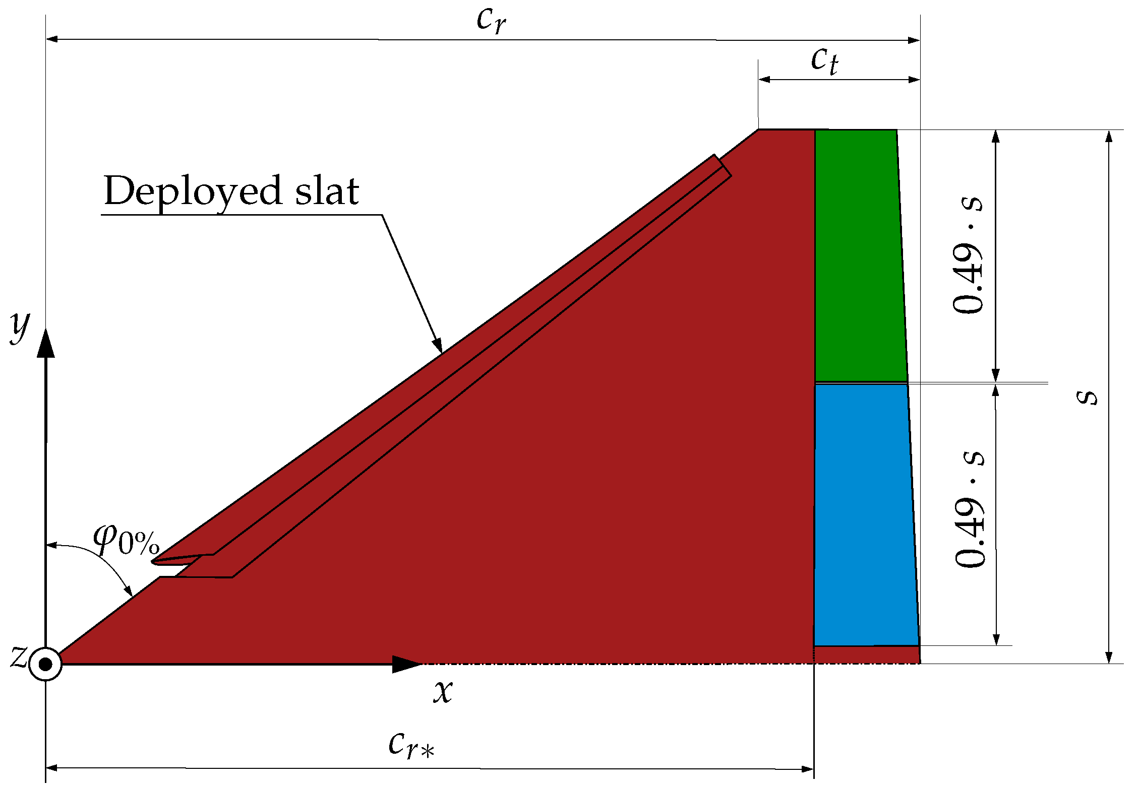
The investigated full-scale wing is a fictive, highly maneuverable cropped delta wing configuration based on the work of Moioli et al. [11]. This design allows for an optimised combination of high lift production and maximum agility [12]. Figure 1 shows the geometric shape of the so-called Model53 as well as the location of the control surfaces at the trailing edge and the position of the aerodynamic frame of reference. This design features a leading edge sweep angle of . A leading edge slat is deployed at an angle of 20°. Besides that, the aspect ratio of the respective wing amounts to , while the taper ratio takes a value of . A continuous wing twist distribution is present, ending up at a 4° twisting angle at the wing tip. Additional dimensions of the wing are listed in Table 1.
2.1. Structural Layout of the Full-Scale Wing
The structure of the wing consists of 5 ribs, a tip rib, a root section, 12 spars, and a trailing edge spar, which are covered by the skin. The control surfaces can be divided into an outer and an inner flap. Each control surface is modelled by 7 ribs and 5 spars, which are covered by a skin. All structural components of the wing and the flaps are ideally connected and modelled by an aluminium alloy 7178 with an elastic modulus and a material density of [13]. The whole geometry with a hidden skin surface is presented in Figure 2a. Here, the locations of the ribs and spars as well as a spike at the rear inboard section of the wing are visualised. An elastic connection between the wing and the flaps is realised by applying a hinge concept between the flaps and the wing according to Reinbold et al. [14]. Each flap is connected to the wing via four hinges, while each hinge consists of two triangular components. One side of the first triangle is directly connected to a flap’s front spar, and one side of the second triangle is clamped at the wing’s trailing edge. The remaining free corner of the first triangle is interconnected with the free corner of the opposing triangle by a rigid bar element (RBE), which is able to transfer moments and forces between the wing and the flap. The RBE of each hinge element lies on the rotational axis of the particular control surface. Figure 2b presents the hinge concept at the inner flap.
For the wing without the flaps, the following properties are assumed. The thickness for all ribs is identical as is the thickness for each spar element. The thickness of the trailing edge of the wing is enlarged with respect to the thickness of the remaining spars. Between two ribs, the skin thickness is assumed to be constant. However, the thickness of the skin decreases in equally spaced, discrete steps towards the wing tip. Therefore, the skin thickness can be described by defining the thickness at the root and at the tip . A similar setup is chosen for the flaps. However, the skin thickness is constant for each flap. The thickness of the triangular hinge elements is identical to the thickness of the wing’s ribs. Nonetheless, it has to be noted that a variation of the hinge thickness can be used to adapt the stiffness of the connection. Table 2 shows the thickness of each structural component for the wing and the flaps.
2.2. Flight Conditions of the Full-Scale Model
This work focuses on the study of the delta wing at a Mach number of for high angles of attack with the aid of a deployed leading edge slat. Furthermore, the full-scale model is simulated at a low flight altitude of [15,16]. As a result, the calculations for the full-scale wing are conducted for an air density of and a static temperature of . These data are based on the standard conditions at mean sea level (MSL) and accounting for the difference in real and geopotential height. The dynamic pressure is calculated based on the according velocities and the respective air density. The Reynolds number is referred to the mean aerodynamic chord . These flow data for the full-scale model can be taken from Table 3.
3. Wind Tunnel Model Application
The development of an elastically scaled configuration is aimed in this work with the purpose of constructing an applicable wind tunnel model design. Therefore, the fictive, full-scale configuration is taken as a reference case. The dimensions of the outer mould line of the respective wind tunnel model are scaled down by a factor of . The respective dimensional data of the wind tunnel model are given in Table 1. To achieve a structural similarity between the full-scale and the scaled configuration, the nondimensional location of the structural elements of the scaled configuration is identical with respect to the full-scale setup. Nevertheless, the thicknesses of the wind tunnel model elements need to be optimised to fit the structural characteristics of the full-scale model. Unlike the full-scale version, the wind tunnel model is made out of polypropylene by stereolithographic (SLA) printing. This printing method ensures the construction of a pseudo-monolithic part with a high level of microstructural isotropy [17]. The material Xtreme White 200 is chosen as an appropriate plastic. This material exhibits a mean elastic modulus of and a density of in the cured state [18]. The different material choice with respect to the full-scale wing has to be taken into account for the optimisation process as well.
3.1. Wind Tunnel Conditions for the Scaled Model
Contrary to the full-scale configuration, the wind tunnel model is investigated at mean sea level (MSL) conditions. As a result, the air density amounts to . The air speed for the wind tunnel model is calculated, originating from the true air speed of the full-scale wing, implying a Froude number similarity with . The dynamic pressure is calculated analogously to the procedure for the full-scale model. The flow data for the scaled configuration can be taken from Table 3.
3.2. Scaling Methodology
The adequate component thicknesses of the scaled model are determined using a specifically designed MATLAB [19] tool. For the optimisation procedure, the delta wing configuration is split up into its main components, the wing and the two flaps, which are then optimised separately. Applying this code, a structural grid is generated for a full-scale component and its analogous scaled part. For further references, the configuration without the flaps will be called wing, and a combination of the wing and flaps will be referred to as a full-scale and scaled model or configuration. Furthermore, a plane setup is used for the modelling of the wing and the flaps. Ribs and spars are modelled via a beam approach [20], while the skin is modelled by shell elements [21,22]. The thickness values from Table 2 are used as an input for the investigated full-scale elements, while variable parameters are utilised for the according thickness values of the scaled component. As the wing and flaps are assumed to be a flat 2D object, the thickness has to be accounted for by including the parallel axis theorem as far as skin shells are concerned. However, the parallel axis theorem only considers the height of the middle line of the skin. Due to the fact that the local skin-thickness-to-wing-thickness ratio takes on a considerable value, the offset of the middle line of the skin to the components’ surface has to be included into the calculations. The according mass of each structural element is equally split up and assigned to the adjacent nodes as lumped masses. As a result, the stiffness and mass matrix can be computed for a full-scale component and its according scaled component. However, the matrices for the scaled component will contain variables for the thickness of the ribs, spars, and skin. Subsequently, these thickness values are varied until identical structural characteristics are achieved between the scaled and the full-scale component.
To reduce the order of complexity, the wing was investigated without the spike. The wing’s structural grid is meshed with 13 nodes in spanwise direction and 27 nodes in chordwise direction (see Figure 3). Each structural node has one translational and two rotational degrees of freedom, which sums up to a total number of degrees of freedom, excluding the Dirichlet boundary nodes at the wing root, where the wing is assumed to be clamped. The setup for both flaps is chosen accordingly. Each flap is meshed by 13 nodes in spanwise direction and 9 points in chordwise direction. For this approach, the flaps are assumed to be clamped at the respective hinge line.
3.2.1. Fundamental Scaling Laws
To accomplish a dynamic similarity between the full-scale and the scaled model, multiple factors need to coincide according to the transformed equation of motion (A14), which is shown in Appendix A. An optimisation of the rib, spar and skin thicknesses of the scaled model is used to fit these criteria. The necessary factors are listed below [23]:
- The nondimensional modal mass matrix ;
- The nondimensional modal frequencies ;
- The nondimensional mode shapes ;
- The reduced angular frequency of the first mode ;
- The inertia ration ;
Additionally, the aerodynamic shape of the scaled model and the full-scale wing have to be equivalent. To achieve similar flow properties, a Reynolds number and Mach number M similarity is necessary in order to obtain equivalent flow conditions. However, a mismatch for these two criteria cannot be avoided for the scaled model in a practical application in a typical low-speed wind tunnel facility, such as wind tunnel A at the Technical University of Munich [26]. Then, the main focus will be on the matching of the nondimensional modal frequencies and the the nondimensional mode shapes in particular.
3.2.2. Stiffness Matrix Fitting
As the mass and stiffness matrix of a scaled component contain variables for the rib, spar, and skin thickness, the stiffness matrix of a scaled component is optimised for a static load condition at first. Therefore, the occurring deformation of the full-scale component is calculated for an aerodynamic loading, which is determined for a given aerodynamic angle of attack by using the vortex lattice method (VLM). A plane aerodynamic grid representing the outer mould line of the investigated component is utilised for the generation of a representative aerodynamic load vector. As the grid size of the structural grid and of the aerodynamic grid differs, a force transfer between collocation points of the vortex lattice mesh and the nodes of the structural grid is necessary [27]. In case of a force transfer from the aerodynamic surface mesh to the structural nodes, a nearest-neighbour search, the so-called point-element relationship, is applied. This search method assigns the aerodynamic load in each collocation point of the aerodynamic mesh to the closest node in the structural mesh. Using this method, a conservative interpolation with regard to moment and force balance is ensured [28]. As a result, a load matrix for the full-scale component is obtained, which contains the aerodynamic forces and moments . The computed translational deformation of the full-scale component can be scaled down by the factor , while the rotational deformation stays unaltered, to attain the equivalent deformation of the scaled component . Hereby, an identically scaled deformation is predefined for the scaled part. The forces and moments at each node of the full-scale component can be transferred to the equivalent nodes of the scaled component by reducing the forces by the factor and the moments by the factor . In this regard, the connectivity between the full-scale load and the scaled load can be defined by the force ratio as follows [29]:
Here, quantifies the air density ratio between the scaled and full-scale configuration, while analogously resembles the flow velocity ratio. A fixed Froude number for the full-scale and the scaled model sets the velocity ratio to . This definition of the force ratio ensures an equivalent transmission of the load distribution from the full-scale to the scaled component. As a result, an identical distribution is defined along the dimensionless coordinates and of a scaled and a full-scale component. According to dimensional analysis, a transmission of moments to a scaled component by the factor can be conducted as depicted in Equation (2) [30].
The transformation matrices and for the load vector and the deformation vector for a full-scale component yield the following forms:
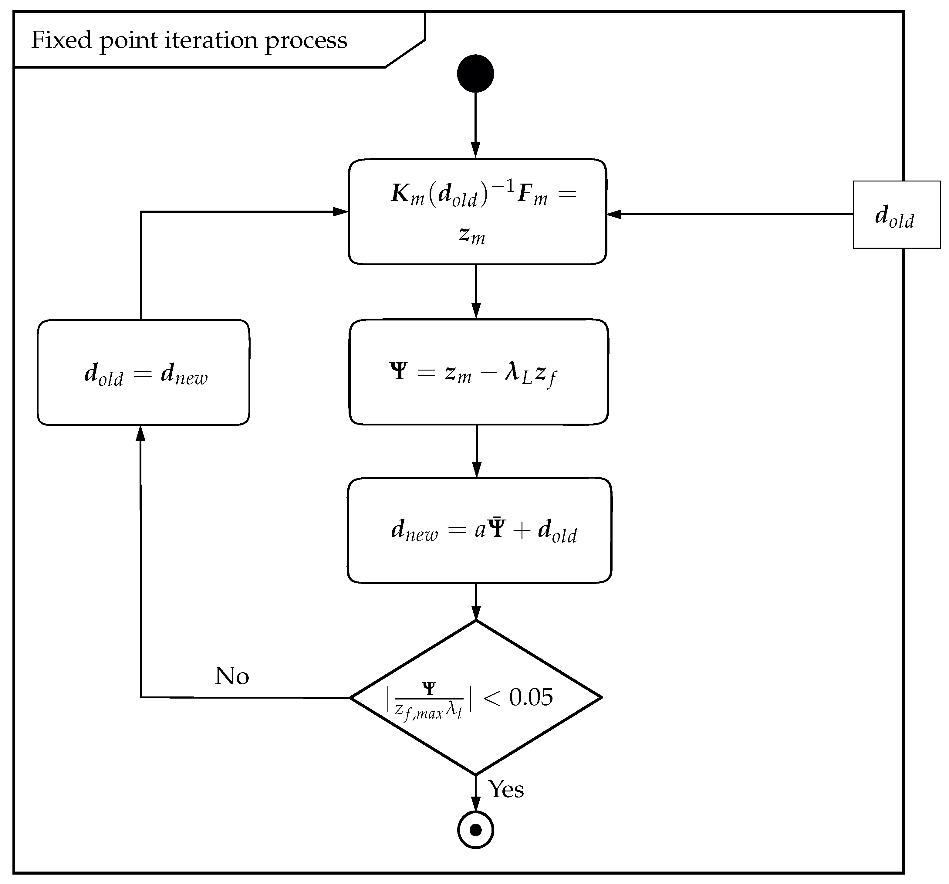
With the known applied model loads and resulting model deformations, the scaled component stiffness matrix can be optimised. Therefore, a fixed-point iteration is applied according to the flowchart diagram depicted in Figure 4. The optimisation starts from a given starting vector , which resembles the parameters for the wall thickness of all structural elements of a scaled component, and proceeds until a local minimum of the objective function is reached. Due to the fact that the number of nodes of the structural grid is larger than the number of parameters, only a reduced number of collocation points are used to calculate the next iteration step of the thickness parameters . Additionally, an acceleration factor a can be applied to speed up the convergence behaviour. For the case of convergence, the relative deviation between the deformation of the scaled component and the downscaled deformation of the full-scale component of each grid point i satisfies the condition , and the iteration queue is stopped. Hereby, defines the downscaled maximum deformation of the investigated full-scale component.
3.2.3. Mass Matrix Fitting
With the stiffness matrix of a scaled component defined, the mass matrix needs to be optimised in order to achieve dynamic similarity with the equivalent full-scale component. A predefined number of lumped masses with unknown values at distinct locations in the configuration are used to modify the dynamic behaviour of a component and tune the eigenvalues and eigenvectors of the system. Figure 5 depicts the optimisation process for the model mass matrix. Starting from the fixed stiffness matrix and the according mass matrix of the scaled component, the normalised eigenvector matrix and the eigenvalues of a full-scale component are utilised to calculate the needed additional masses for the scaled component. The target eigenvector matrix of the scaled component is identical to the matrix of the full-scale component, while the target eigenfrequencies of the model are calculated using the scaling law . For the calculation of the matrix , eigenvalues are taken into account. Using a minimum search for the objective function, the additional masses are computed. A finite number of the first eigenfrequencies are used to define the objective function . Afterwards, the true eigenfrequencies and normalised eigenvector matrix of the scaled component can be determined.
3.3. Structural Data Fitting for the Wing and Flaps
The optimised relevant thicknesses of the structural elements of the wing design and the flaps are given in Table 4. All calculated thicknesses are independent from the flow velocity, which permits a representation of the full-scale configuration at a fixed altitude by one wind tunnel model only. With the calculated thicknesses of the scaled model, the aeroelastic characteristic can be defined by the nondimensional quantity in Equation (4).
In this regard, the ratio of the dynamic pressure and Young’s modulus of the 3D-printed material is calculated. The thickness of the wing spars is embedded to account for the structurally optimised design of the scaled model. Hereby, the spar thickness is used exemplarily for all optimised quantities, as it is of high significance for the bending characteristic of the wing. The half span of the model is used to nondimensionalise the expression. Analogously, the according value is calculated for the full-scale model in Equation (5). The relative difference between these scaled and full-scale model values amounts to .
3.3.1. Stiffness Matrix and Deformation Matching of the Scaled Wing
As described in Section 3.2.2, the stiffness of the wind tunnel model wing without the flaps is optimised to fit the downscaled deformation of the full-scale wing without flaps for equivalent static load conditions. The relative error between the downscaled deformed full-scale wing and the deformed wind tunnel model wing is calculated according to Equation (6). The maximum deformation of the full-scale wing is used as a reference value. The optimisation process is continued until a convergence to the targeted shape is approached and the relative error of each node j of the grid is below . Figure 6 shows the relative error surface regarding the deviation of the scaled wing with respect to the target deformation at a Mach number . The maximum absolute value of occurs at of the half span.
3.3.2. Eigenmode and Eigenfrequency Analysis of the Scaled Wing
After the optimisation process of the stiffness matrix, the mass matrix of the wind tunnel model wing is known, and an optimisation of the mass matrix is conducted by adding lumped masses in distinct positions. These locations are shown in Figure 3. However, the optimisation process described in Figure 5 yields that for the particular setup, no improvement of the eigenvalue problem is necessary for a maximum deviation of from the targeted eigenfrequencies. The output of the eigenvalue problem performed using the MATLAB tool is listed in Table 5. Here, the first five modes of the full-scale wing and the wind tunnel model wing are investigated with respect to their eigenfrequencies. Furthermore, the reduced angular frequency is given for the full-scale wing and, respectively, for the wind tunnel model wing for each mode i. The relative difference of these two values is also listed for each mode. From mode 1 to mode 5, the relative difference is between and .
Furthermore, the first three mode shapes of the wind tunnel model wing, including the deviation of each mode shape from the respective targeted shape of the full scale wing, are depicted in Figure 7. The deviation of the points j of each mode i is calculated according to Equation (7). Here, the value in the denominator represents the maximum value in the i-th column of the normalised matrix with . Figure 7a shows the first mode shape of the wind tunnel model wing. A bending characteristic is primarily attributed to this shape. The according deviation of this mode shape with respect to the mode shape of the full-scale wing is shown in Figure 7b. A maximum deviation of is visible in the leading edge region of the wing at . A moderately increased deviation of can also be determined at the trailing edge in the inner wing section (). The mode corresponding to the second eigenfrequency can be seen in Figure 7c. This mode visualises a coupled twisting and bending nature. The graph features a twist along the wing span with an increasing bending characteristic of the wing towards the tip. The deviation plot of the second mode points out the maximum negative values of at at the leading edge, while the positive maximum of is located at . The third mode (Figure 7e) shows a further twisting characteristic of the wing. Contrary to the second mode, the global maxima of the shape are located in the midwing section at of the half span and at the leading edge of the wing tip. The deviation regarding this mode is plotted in Figure 7f. The highest recorded deviation of is detected at on the leading edge.
At last, the inertia ratio of both the wind tunnel model wing and the full-scale wing is compared. The inertia ratio of the full-scale wing takes on a value of , while the value of the wind tunnel model wing amounts to . As a result, the relative difference between the two values is . This value is larger than the relative difference of the reduced frequencies listed in Table 5. Furthermore, it is larger than the relative differences between the mode shapes, as the inertia ratio is only indirectly optimised. A comparison of the diagonalised nondimensional modal mass matrix of the scaled and the full-scale wing shows a relative deviation below for the first five entries.
3.3.3. Flap Optimisation
The separate static optimisation of the flap thicknesses with the resulting values from Table 4 yields a maximum deviation of the targeted shape below for both flaps. Furthermore, a proper coalescence between the reduced frequency of the full-scale flaps and the flaps of the scaled model is achieved. The eigenfrequency analysis for the first three modes for the inner flap is shown in Table 6. Analogously, the first three eigenfrequencies of the outer flap are given in Table 7. For both flaps, a relative difference is achieved for all eigenfrequencies. Furthermore, the relative difference between the inertia ratios of the full-scale flaps and the wind tunnel model flaps is kept below for both flaps.
4. Aerodynamic Simulations
4.1. Simulation Setup
In order to evaluate the assumption regarding a similar pressure coefficient distribution for the scaled and the full-scale configuration from Section 3.2.2, high-fidelity steady-state computational fluid dynamics (CFD) calculations are performed for a half-model geometry. Therefore, the aerodynamic data from Table 3 are investigated. The simulations are carried out using Ansys Fluent [32] to solve the compressible, three-dimensional Reynolds-averaged Navier–Stokes (RANS) equations. The RANS equations are closed with the two-equation turbulence model. Regarding the pressure-based solution method, a pressure–velocity coupling is applied. The coupled algorithm solves the momentum and pressure-based continuity equations collectively [33]. This coupling procedure is performed by an implicit discretization of pressure gradient terms in the momentum equations and an implicit discretization of the face mass flux, including the Rhie–Chow pressure dissipation terms [34]. A second-order upwind scheme is utilised for the spatial discretisation. Furthermore, a global pseudo–time step is used for the stabilisation of the steady-state calculations. An adequate time step is chosen to achieve an optimum trade-off between fast convergence time and result accuracy. The according study is shown in Figure 8a. For the following calculations, the intermediate pseudo–time step of is applied for the scaled configuration. Analogously, the intermediate pseudo–time step of is used for the full-scale configuration. During the pre-processing, a poly-hexcore hybrid meshing technique is used to generate the volume grid for the full-scale and the scaled wing. Using this approach, hexahedral cells are generated in the bulk region, while polyprisms are used to model the boundary layer. A mosaic technology is applied to link these two regions [35]. A semispherical pressure farfield with a diameter of is chosen for the full-scale wing and, respectively, for the scaled wing. The plane surface of the semisphere resembles the symmetry plane of the setup. Additional refinement areas are defined in the vicinity of the wing. A grid sensitivity study is conducted for four grid refinement levels for the full-scale and the scaled configuration. An extreme coarse, a coarse, a medium, and a fine grid are investigated. The cell size is refined by a factor of for each grid refinement step. As a result of the study, which is depicted in Figure 8b, the medium grid is rated as sufficiently resolved for the full-scale and the scaled configuration and chosen for further calculations. The medium grid of the scaled configuration has a total cell count of , while a higher cell count is reached for the full-scale application with cells. The polyprism layers of the medium grid of the scaled model are created by applying a uniform offset method with 40 layers and a growth rate of . With a first-layer height of , a low wall treatment of is aimed to resolve the boundary layer. Analogously, 40 polyprism layers with a growth rate of are utilised for the medium grid of the full-scale model. A first-layer height of is applied to fulfil the requirement. For the grid generation during the grid sensitivity study, the total layer height is fixed, which leads to a variation of the layer number and the growth rate for a varying first-layer thickness. Figure 9 presents the structure of the full-scale and the scaled grids.
4.2. Aerodynamic Coefficients
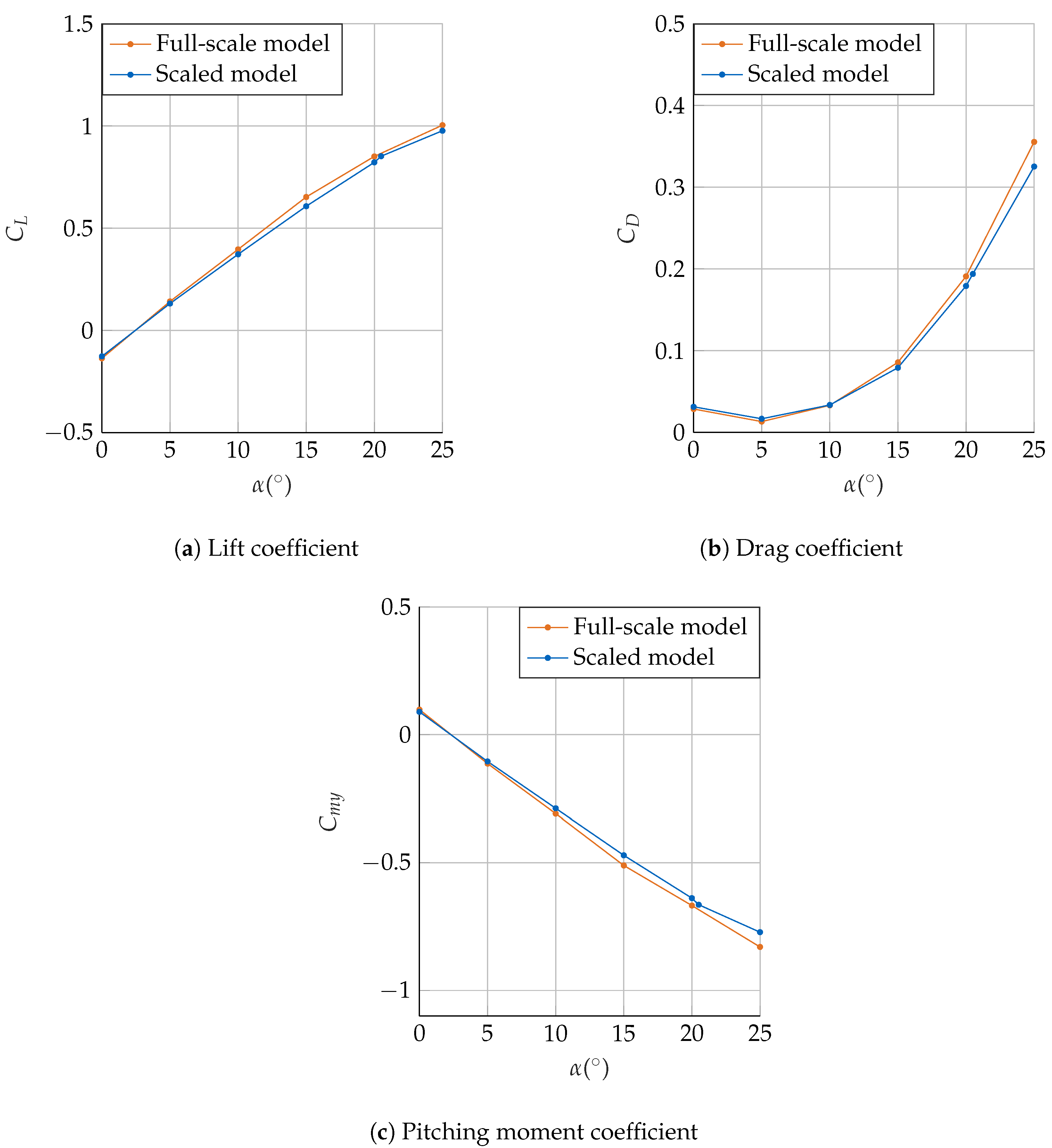
The global aerodynamic coefficients for the scaled and the full-scale model are given in Figure 10. Therefore, the full-scale wing is studied at a Mach number of , while the Mach number of the scaled wing amounts to . However, the Froude number for both cases is identical. For the angle of attack, an interval from 0° to 25° is investigated in 5° steps. Figure 10a pictures the lift coefficient for the scaled and the full-scale wing. For low angles of attack up to , both curves are almost identical. Towards higher angles of attack, the differences between the two curves increase due to compressibility effects on the full-scale wing. The lift continuously increases towards the maximum investigated angle of attack of for both setups. However, the lift curve slope starts to decline for angles of attack greater than . At , the relative difference between the lift coefficient of the scaled and the full-scale model is . An angle of attack of is additionally investigated for the scaled model with a lift coefficient of to match the global lift coefficient of the full-scale model with a reduced relative difference of . Considering the drag coefficient in Figure 10b, the curves of the scaled and the full-scale wing coincide up to an angle of attack of . The minimum drag coefficient of for the scaled wing and for the full-scale wing occurs at . For angles of attack greater than 10°, the drag coefficient of the full-scale model exceeds the values for the scaled model. A relative difference between the scaled and the full-scale model of occurs at . Furthermore, the pitching moment coefficient is visualised in Figure 10c. The according moment reference point is chosen at the apex of the wing. Therefore, the mean aerodynamic chord is used as the reference lever arm. From to , the coefficients of the scaled and the full-scale models follow a similar trajectory. Between and , the full-scale configuration exhibits a smaller value of the pitching moment coefficient with respect to the wind tunnel model. For , the relative difference between the scaled and the full-scale model amounts to .
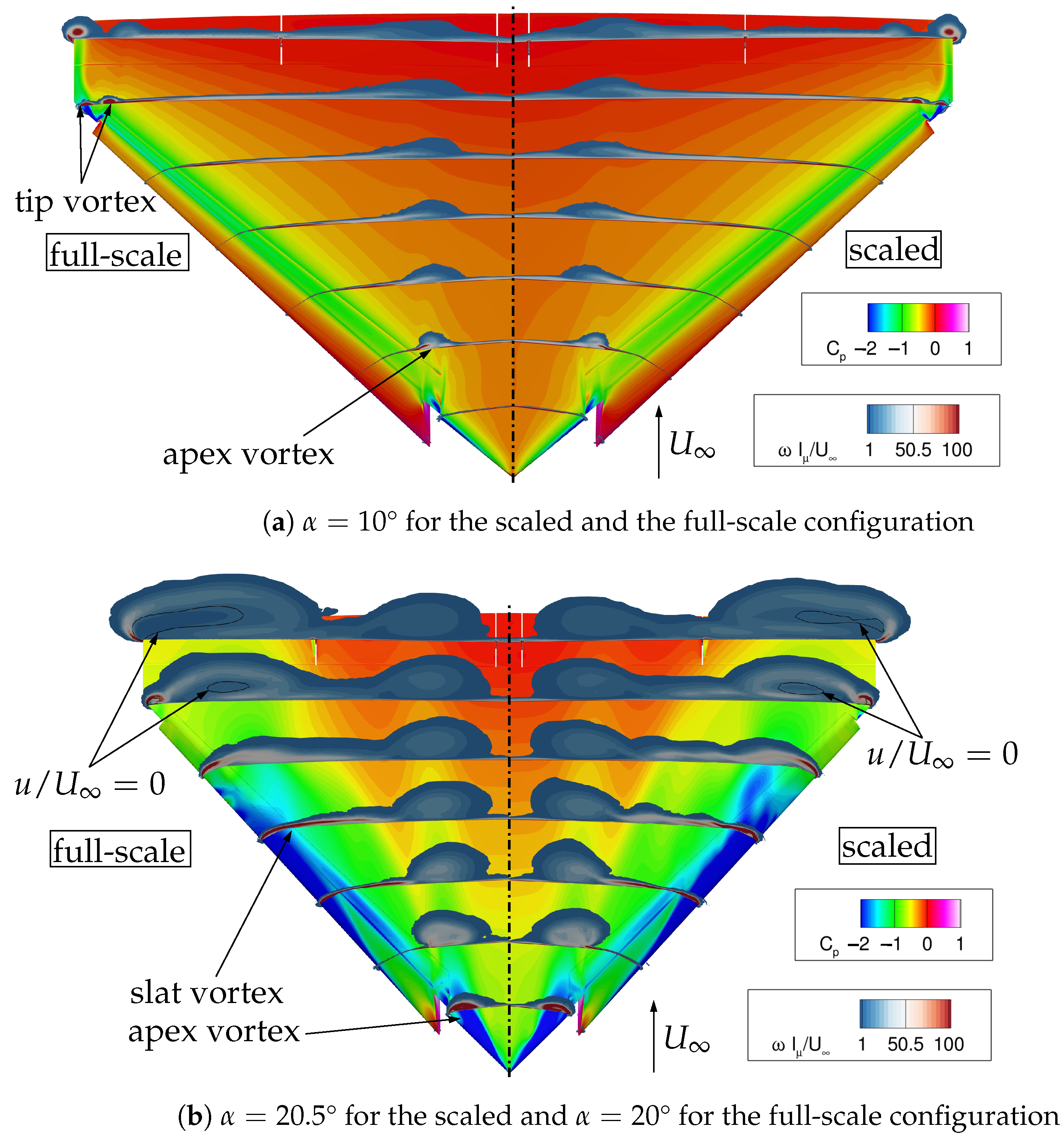
A detailed analysis of the local aerodynamics is shown in Figure 11. Figure 11a shows the distribution on the upper side of the scaled model and the full-scale configuration for an angle of attack of . Furthermore, seven cross-flow planes are shown, which visualise the normalised vorticity field . These planes enable the identification of a weak leading-edge vortex originating at the apex and a tip vortex system, which is triggered at the leading edge outboard of the slat for both models. Furthermore, a local pressure minimum occurs at the intersection between the slat and the wing for the scaled and the full-scale wing. Minor differences between the distribution of the full-scale and the scaled model are visible at the root section between and of the local chord. The overall distribution shows a similar characteristic. Figure 11b pictures the characteristics of the scaled model at and of the full-scale model at . This particular setup is chosen to aim for an equivalent pressure coefficient distribution on the wing’s surfaces and an identical global lift coefficient, which is a necessary criterion for a dynamic similarity of the full-scale and the scaled model, according to Section 3.2.2. With respect to the lower angle of attack of , the apex vortex is pronounced more strongly for both models. The influence of the vortex reaches far downstream to the inner flap. Furthermore, a second vortex is observable at the deployed slat. This vortex is carried downstream to the outer flap. However, for this vortex, a region of reversed flow can be identified in the rear section of the wing. This phenomenon indicates a bursting of the vortex at this angle of attack. The scaled model and the full-scale model show a similar flow topology across the wing and flaps.
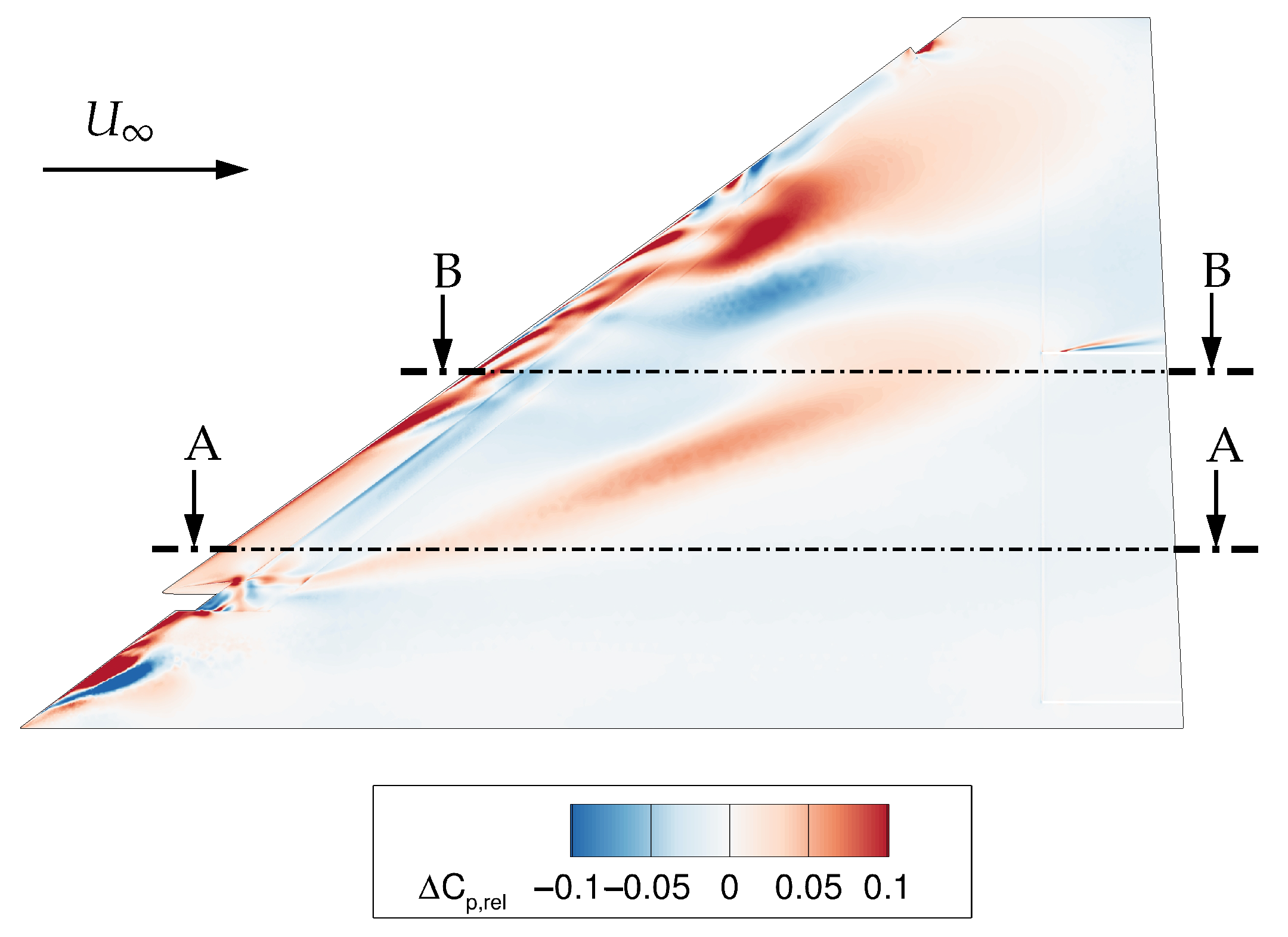
For a more detailed investigation of the aerodynamic differences between the scaled model at and a Mach number of and the full-scale model at and a Mach number of , the relative pressure coefficient deviation according to Equation (8) is shown in Figure 12. Here, describes the local pressure coefficient of the scaled model, and represents the local pressure coefficient of the full-scale configuration. An area with high positive and negative values occurs near the apex. This indicates a bending of the apex vortex core of the scaled wing towards the leading edge with respect to the full-scale apex vortex. This difference, however, will have no major impact on the static deformation of the wing due to the small lever arm with respect to the wing root. A second region with increased absolute values of arises between and of the respective half span of the delta wing. The low-pressure field of the scaled wing, which is created by the second vortex originating from the deployed slat, reaches further downstream compared with the equivalent vortex of the full-scale wing. Furthermore, this slat vortex core of the scaled wing is shifted towards the wing root with respect to the full-scale wing, which additionally leads to a deviation of the aspired values in that area. In the wing tip region, relative differences in the distribution of appear due to minor differences in the flow topology and location of the second occurring vortex. In contrast to that, low values for occur at the root and trailing edge.
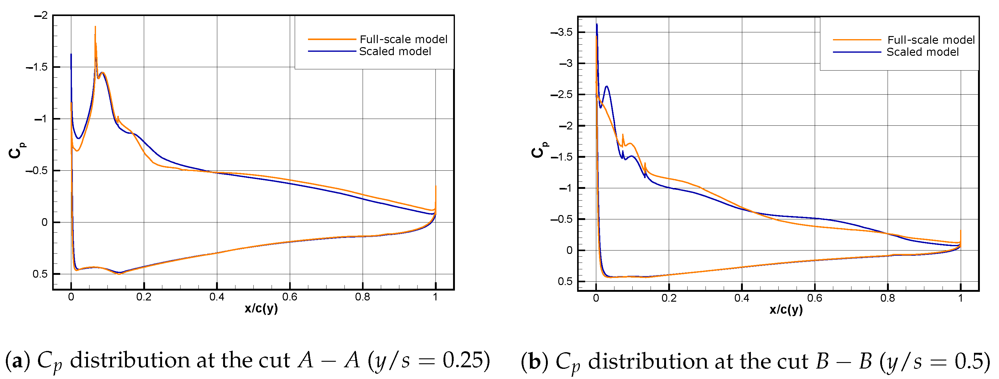
Two surface cuts, and , are positioned in Figure 12. The cut is located at , while represents a surface cut at . The pressure coefficient curves at these cuts are shown in Figure 13. Figure 13a reveals a difference in the plot between the scaled and the full-scale wing’s upper side between and of the local chord length. For the second surface cut (), a positive difference between the distributions of the scaled and the full-scale model can be identified between and of the local chord. From to of the chord, a negative difference between the distributions of the scaled and the full-scale model occurs. However, for a wide area of the wings’ surface, the scaled and the full-scale wing show a matching of the pressure distribution, in particular, at the leading edge, trailing edge, and lower side of the wing.
5. Finite Element Analysis of the Model53 with Integrated Flaps
5.1. Structural Grid Resolution
To verify the results of the optimisation procedure conducted with the MATLAB tool, the finite element code ELFINI, implemented in CATIA, is utilised. Therefore, the structural characteristics of the entire model with integrated flaps according to the description in Section 2.1 are analysed. The values for the wall thickness of the skin, spars, and ribs are used to generate a three dimensional CAD model of the full-scale and the scaled model. All structural elements are modelled by two-dimensional shell elements. The structural grid of the scaled wind tunnel model consists of triangular elements with a reasonably small mean side length of . The total count of elements amounts to . Similarly, a shell structure is generated for the full-scale model as a reference case. Therefore, an equivalent element size of is chosen. As a result, elements are generated. For the structural analysis of both cases, the wing is clamped at the root chord.
5.2. Frequency Analysis
Table 8 presents the results of the frequency analysis. Here, the first five eigenfrequencies of the full-scale model and the wind tunnel model are presented. Determining the relative difference between the reduced frequencies of the scaled and the full-scale configuration yields a value of for the first eigenfrequency, followed by for the second frequency. The absolute discrepancy for the following three frequencies is below 2.5%.
5.3. Mode Shape Analysis
In addition to the analysis of the eigenfrequencies, the according normalised mode shapes of the full-scale and the scaled wing are analysed in Figure 14. The plotted colour bar resembles the absolute deformation with respect to the nondeformed state of the model. Figure 14a shows the first bending mode of the full-scale model and the scaled model corresponding to the first reduced frequencies and . The mode shape of the full-scale model is presented on the bottom half of the picture, while the mode shape of the scaled model is shown on the top half. Figure 14b shows the first twisting mode of the full-scale and the scaled Model53 at the reduced frequency . This frequency contains a large contribution of the inner flap movement around its hinge axis. The third mode shape is given in Figure 14c and shows the second twisting characteristic. However, an increased contribution of the outer flap motion is characterised at this frequency . The second bending mode can be identified at the fourth reduced frequency , which is shown in Figure 14d. The fifth natural frequency has a twisting characteristic and is presented in Figure 14e. For all five reduced frequencies, the mode shapes of the scaled model and the full-scale configuration show a high similarity across the entire model surface. Furthermore, Figure 14 shows a visible movement of the inner and outer flap with respect to the main wing, which enables the capturing of aeroservoelastic effects of the flaps.
5.4. Deformation Analysis
Furthermore, a deformation analysis is conducted using the ELFINI FEM model of the scaled and full-scale configuration and by applying the calculated aerodynamic loads from the CFD simulations. Figure 15 shows the normalised deformation in z-direction of the structure of the scaled model on the top half and of the full-scale model on the bottom half. The normalisation of the deformation in z-direction is conducted using the half span s of the according model. For the scaled model, the aerodynamic forces at and an angle of attack of are considered. The resulting forces at and an angle of attack of are used for the full-scale model. A maximum normalised deformation of arises at the trailing edge of the tip for the scaled configuration, while a maximum of can be determined for the full-scale model in the same region. Thus, the relative difference between the maximum normalised deformation of the scaled and the full-scale model is . The overall shape of the deformation shows a high degree of similarity for both models.
6. Conclusions
This work explains the development of an aeroelastic scaling procedure for the wing and flaps of a fictive delta wing configuration intending to design a concept for a wind tunnel application. The optimisation procedure of the scaled model wing and the flaps, using adequate scaling laws, yields thicknesses for the ribs, spars, and skin at a magnitude of a few millimetres. The optimisation is conducted by fitting the stiffness matrix of a scaled component and adjusting the resulting mass matrix to attain the targeted values for the eigenfrequencies. The procedure shows that no additional masses are needed to achieve a desired maximum deviation of with respect to the targeted first three eigenfrequencies of a component. In addition to the structural requirements for the aeroelastic similarity between the full-scale and the scaled model, the aerodynamic similarity is investigated using Ansys Fluent. A comparison of the global aerodynamic coefficients between the scaled and the full-scale model shows an increasing difference towards the maximum investigated angle of attack of for the drag and moment coefficient. The curves for the lift coefficient show a minor relative deviation across the whole angle of attack interval. A local comparison between the flow phenomena of the scaled and the full-scale wing at an angle of attack shows a high level of similarity in the pressure coefficient distribution and normalised vorticity magnitude at different cross-flow planes. Additionally, the reference case of the full-scale model at is compared with for the scaled model to achieve a minimal deviation of the global lift coefficient. Locally, the pressure coefficient distribution shows relative deviations up to between and of the half span due to a different location of the slat-induced vortex system. However, for a large wing surface area, the pressure coefficient deviation is kept close to . A following verification of the structural optimisation of the scaled configuration reveals a maximum deviation of from the first five targeted eigenvalues, which occurs for the second eigenfrequency. Furthermore, the according investigated mode shapes show a high level of similarity. At last, a comparison of the normalised deformation in z-direction between the scaled and the full-scale model is presented. Therefore, the aerodynamic calculations for and are applied to the structural grid of the full-scale model. For the scaled model, the simulation results for and are applied to the according structural grid. The maximum deformation occurs at the trailing edge of the wing tip for both models. The relative difference between the maximum deformation of the scaled and the full-scale model amounts to . These results confirm the accuracy of the optimisation process. All in all, the scaling procedure of the investigated delta wing shows an adequate resemblance to the fictive full-scale wing.
Author Contributions
K.B.: conceptualization, formal analysis, investigation, methodology, software, validation, visualization, writing—original draft; C.B.: conceptualization, supervision, writing—review and editing. All authors have read and agreed to the published version of the manuscript.
Funding
This research received no external funding.
Data Availability Statement
The data presented in this study are available on request from the corresponding author.
Acknowledgments
The authors want to thank ANSYS for providing the flow simulation software.
Conflicts of Interest
The authors declare that they have no known competing financial interests or personal relationships that could have appeared to influence the work reported in this paper.
Abbreviations
The following abbreviations are used in this manuscript:
| Greek Symbols | |
| angle of attack | |
| first Rayleigh coefficient | |
| second Rayleigh coefficient | |
| relative error between the mode shape of the full-scale and the scaled wing | |
| aspect ratio | |
| eigenvalue | |
| force scaling factor | |
| geometrical scaling factor | |
| moment scaling factor | |
| taper ratio | |
| velocity scaling factor | |
| normalised modal frequency matrix | |
| modal frequency matrix | |
| inertia ratio | |
| density | |
| material density of aluminium and SLA | |
| nondimensional time | |
| rotation angle of the j-th node around length axis | |
| rotation angle of the j-th node around lateral axis | |
| sweep angle at the leading edge | |
| nondimensional deformation vector | |
| nondimensional mode shape matrix | |
| Latin Symbols | |
| relative difference between the pressure coefficient of the full-scale and | |
| the scaled model | |
| relative difference between the i-th reduced angular frequency of the | |
| full-scale and the scaled model | |
| time step size | |
| deformation in z-direction | |
| deformation in z-direction for the full-scale and the scaled model | |
| normalised modal mass matrix | |
| modal damping matrix | |
| modal stiffness matrix | |
| modal mass matrix | |
| uniformly dimensionalised damping matrix | |
| uniformly dimensionalised stiffness matrix | |
| uniformly dimensionalised mass matrix | |
| aerodynamic damping matrix | |
| aerodynamic stiffness matrix | |
| aerodynamic mass matrix | |
| damping matrix | |
| stiffness matrix | |
| mass matrix | |
| mode shape matrix of the full-scale and the scaled model | |
| transformation matrix | |
| deformation vector | |
| b | span |
| drag coefficient | |
| lift coefficient | |
| pressure coefficient | |
| root chord | |
| tip chord | |
| pitching moment coefficient | |
| pressure coefficient of the full-scale and the scaled model | |
| root chord without the spike of the full-scale and the scaled model | |
| root chord without the spike | |
| root chord of the full-scale and the scaled model | |
| tip chord of the full-scale and the scaled model | |
| Young’s modulus for aluminium and SLA-printed material | |
| F | force |
| f | eigenfrequency |
| i-th eigenfrequencies of the full-scale and scaled model | |
| Froude number | |
| Froude number for the full-scale and the scaled wing | |
| g | gravitational constant |
| h | flight altitude |
| i-th reduced angular frequency | |
| i-th reduced angular frequency of the full-scale and the scaled model | |
| mean aerodynamic chord | |
| mean aerodynamic chord of the full-scale and the scaled model | |
| M | Mach number |
| m | moment |
| n | total number of degrees of freedom |
| q | dynamic pressure |
| dynamic pressure of the full-scale and the scaled model | |
| Reynolds number | |
| Reynolds number of the full-scale and the scaled model | |
| s | half span |
| half span of the full-scale and the scaled wing | |
| wing reference area of the full-scale and the scaled model | |
| wing reference area | |
| T | temperature |
| rib thickness of the full-scale model | |
| skin thickness of the full-scale model at the root | |
| skin thickness of the full-scale model at the tip | |
| spar thickness of the full-scale model at the trailing edge | |
| spar thickness of the full-scale model | |
| rib thickness of the scaled model | |
| skin thickness of the scaled model at the root | |
| skin thickness of the scaled model at the tip | |
| spar thickness of the scaled model at the trailing edge | |
| spar thickness of the scaled model | |
| inflow velocity of the full-scale and the scaled model | |
| inflow velocity | |
| x | x-coordinate of the aerodynamic frame of reference |
| y | y-coordinate of the aerodynamic frame of reference |
| z | z-coordinate of the aerodynamic frame of reference |
Appendix A. Scaling Methodology
In order to derive a structurally dynamic similarity relation between the scaled model and the full-scale configuration, the linear elastic equation of motion, depicted in Equation (A1), is utilised. Then, a general concept for the structural analysis of arbitrary systems—the scaled model and the full-scale model likewise—as well as the criteria for dynamic structural similarity, is introduced.
Here, , , and symbolise the mass, damping, and stiffness matrices of the system, while , , and resemble aerodynamic mass, damping, and stiffness equivalent terms. The vector characterises the gravitational acceleration [23]. The first step to obtain a scale-independent relation is to normalise the deformation vector . As depicted in Equation (A2), consists of one translational and two rotational degrees of freedom for each structural node. The deformation in z-direction and the rotations around the length x-axis and the y-axis are considered.
A nondimensionalisation of is achieved by the multiplication of the transformation matrix . Consequently, the uniformly dimensionalised mass, damping, and stiffness matrices are given in Equations (A4)–(A6). Analogously, the mutated aerodynamic matrices are calculated [36].
For a homogeneous differential equation, an assumed response of the system leads to an equation containing the eigenvectors and eigenvalues of the uniformly dimensionalised system, as shown in Equation (A8).
According to Wright and Cooper [37], the resulting eigenmodes and frequencies will be equivalent to the undamped case if proportional damping is assumed. This simplification is used for the following analysis of the structural eigenfrequencies and modes. As a result, the eigenmodes and values can be calculated by the mass and stiffness matrices only. The vector of modal coordinates and the modal mass, damping, and stiffness matrices , , and are calculated using the matrix of nondimensional mode shapes . To reduce the order of complexity, a shortened number of eigenmodes are used to construct .
Here, specifies an diagonal matrix with the first eigenfrequencies. The modal stiffness matrix can be rewritten using the modal mass matrix and the squared matrix . As stated before, a proportional damping matrix is assumed for the following part. Due to this simplification, the structural damping matrix is decomposed into two terms, which are defined by the modal mass and stiffness matrix as well as two Rayleigh coefficients, and [37].
However, and are not dimensionless. Therefore, the modal mass matrix is normalised by its first entry , and the matrix of eigenfrequencies is normalised similarly by the first modal eigenfrequency . The result is presented in Equation (A14). In this formulation, describes the derivative with respect to a nondimensional time coordinate [38,39].
Equations (A1)–(A14) are valid for the scaled model and the full-scale model. To accomplish an ideal aeroelastic scaling, each factor from Equation (A14) needs to match for the full-scale and the wind tunnel model. However, the nondimensional modal structural damping term of the full-scale and the wind tunnel model cannot be matched arbitrarily, as the factors and depend on the chosen material of the scaled model among other factors. In this regard, Wright and Cooper [37] state that the aerodynamic damping tends to outweigh structural damping. This phenomenon has also been observed for rotating blades by Kielb [40]. For this reason, the structural damping term in Equation (A14) will be neglected for the scaling criteria in this work.
References
- Breitsamter, C. Turbulente Strömungsstrukturen an Flugzeugkonfigurationen mit Vorderkantenwirbeln; Aerodynamik, Utz, Herbert: Munich, Germany, 1997. [Google Scholar]
- Dietrich, H.; Günter, R. Experimentelle Bestimmung der gebundenen Wirbellinien sowie des Strömungsverlaufs in der Umgebung der Hinterkante eines schlanken Deltaflügels; Friedr. Vieweg & Sohn: Braunschweig, Germany, 1971. [Google Scholar]
- Gursul, I.; Xie, W. Interaction of Vortex Breakdown with an Oscillating Fin. AIAA J. 2001, 39, 438–446. [Google Scholar] [CrossRef]
- Mabey, D. Some aspects of aircraft dynamic loads due to flow separation. Prog. Aerosp. Sci. 1989, 26, 115–151. [Google Scholar] [CrossRef]
- Cella, U.; Vecchia, P.D.; Groth, C.; Porziani, S.; Chiappa, A.; Giorgetti, F.; Nicolosi, F.; Biancolini, M.E. Wind Tunnel Model Design and Aeroelastic Measurements of the RIBES Wing. J. Aerosp. Eng. 2021, 34, 04020109. [Google Scholar] [CrossRef]
- Rigby, R.N.; Cornette, E.S. Wind-Tunnel Investigation of Tail Buffet at Subsonic and Transonic Speeds Employing a Dynamic Elastic Aircraft Model. In Report NASA Technical Note D-1362; National Aeronautics and Space Administration: Washington, DC, USA, 1962. [Google Scholar]
- Stenfelt, G.; Ringertz, U. Design and construction of aeroelastic wind tunnel models. Aeronaut. J. 2015, 119, 1585–1599. [Google Scholar] [CrossRef]
- Gibson, F.W.; Igoe, W.B. Measurements of the buffeting loads on the wing and horizontal tail of a 1/4-scale model of the X-1E airplane. In Report NASA Research Memorandum L57E15; National Aeronautics and Space Administration: Washington, DC, USA, 1957. [Google Scholar]
- Tsushima, N.; Nakakita, K.; Saitoh, K. Structural and aeroelastic studies of wing model for transonic wind tunnel test fabricated by additive manufacturing with AlSi10Mg alloys. In Proceedings of the AIAA AVIATION 2022 Forum, Chicago, IL, USA, 27 June–1 July 2022; America Institute of Aeronautics and Astronautics: Reston, VA, USA, 2022. [Google Scholar]
- Katzenmeier, L.; Vidy, C.; Kolb, A.; Breitsamter, C. Aeroelastic wind tunnel model for tail buffeting analysis using rapid prototyping technologies. CEAS Aeronaut. J. 2021, 12, 633–651. [Google Scholar] [CrossRef]
- Moioli, M.; Reinbold, C.; Sørensen, K.; Breitsamter, C. Investigation of Additively Manufactured Wind Tunnel Models with Integrated Pressure Taps for Vortex Flow Analysis. Aerospace 2019, 6, 113. [Google Scholar] [CrossRef] [Green Version]
- Dilger, R.; Hickethier, H.; Greenhalgh, M.D. Eurofighter a safe life aircraft in the age of damage tolerance. Int. J. Fatigue 2009, 31, 1017–1023. [Google Scholar] [CrossRef]
- Aluminium/Aluminum 7178 Alloy (UNS A97178)—azom.com. Available online: https://www.azom.com/article.aspx?ArticleID=6645 (accessed on 15 February 2023).
- Reinbold, C.; Sørensen, K.; Breitsamter, C. Aeroelastic simulations of a delta wing with a Chimera approach for deflected control surfaces. CEAS Aeronaut. J. 2021, 13, 237–250. [Google Scholar] [CrossRef]
- Jebakumar, S.K.; Kumar, N.; Pashilkar, A. Flight Envelope Protection for a Fighter Aircraft. In Proceedings of the 2019 Sixth Indian Control Conference (ICC), Hyderabad, India, 18–20 December 2019; pp. 13–18. [Google Scholar] [CrossRef]
- Liefer, R.K.; Valasek, J.; Eggold, D.P.; Downing, D.R. Fighter agility metrics, research and test. J. Aircr. 1992, 29, 452–457. [Google Scholar] [CrossRef]
- Validierung von Isotropie beim SLA 3D-Druck—formlabs.com. Available online: https://formlabs.com/de/blog/validierung-von-isotropie-beim-sla-3d-druck (accessed on 15 February 2023).
- Accura Xtreme White 200 (SLA) | 3D Systems—3dsystems.com. Available online: https://www.3dsystems.com/materials/accura-xtreme-white-200 (accessed on 15 February 2023).
- Mathworks. MathWorks—Entwickler von MATLAB und Simulink—de.mathworks.com. Available online: https://de.mathworks.com/ (accessed on 15 February 2023).
- Neto, M.A.; Amaro, A.; Roseiro, L.; Cirne, J.; Leal, R. Engineering Computation of Structures: The Finite Element Method, 1st ed.; Springer International Publishing: Cham, Switzerland, 2015. [Google Scholar]
- Ferreira, A.J.M. MATLAB Codes for Finite Element Analysis—Solids and Structures; Springer Science and Business Media: Berlin/Heidelberg, Germany, 2008. [Google Scholar]
- Steinke, P. Finite-Elemente-Methode—Rechnergestützte Einführung; Springer: Berlin/Heidelberg, Germany; New York, NY, USA, 2007. [Google Scholar]
- Ricciardi, A.P.; Canfield, R.A.; Patil, M.J.; Lindsley, N. Nonlinear aeroelastic scaling of a joined-wing aircraft. In Proceedings of the 53rd AIAA/ASME/ASCE/AHS/ASC Structures, Structural Dynamics and Materials Conference, Honolulu, HI, USA, 23–26 April 2012. [Google Scholar] [CrossRef]
- Wan, Z.; Cesnik, C.E.S. Geometrically Nonlinear Aeroelastic Scaling for Very Flexible Aircraft. AIAA J. 2014, 52, 2251–2260. [Google Scholar] [CrossRef] [Green Version]
- Afonso, F.; Coelho, M.; Vale, J.; Lau, F.; Suleman, A. On the design of aeroelastically scaled models of high aspect-ratio wings. Aerospace 2020, 7, 166. [Google Scholar] [CrossRef]
- Wind Tunnel A—epc.ed.tum.de. Available online: https://www.epc.ed.tum.de/en/aer/wind-tunnels/wind-tunnel-a (accessed on 15 February 2023).
- Stickan, B.; Dillinger, J.; Schewe, G. Computational aeroelastic investigation of a transonic limit-cycle-oscillation experiment at a transport aircraft wing model. J. Fluids Struct. 2014, 49, 223–241. [Google Scholar] [CrossRef]
- Keye, S.; Brodersen, O.; Rivers, M.B. Investigation of aeroelastic effects on the NASA common research model. J. Aircr. 2014, 51, 1323–1330. [Google Scholar] [CrossRef]
- Pires, T. Linear Aeroelastic Scaling of a Joined Wing Aircraft; Instituto Superior Tecnico: Lisbon, Portugal, 2014. [Google Scholar]
- Zohuri, B. Dimensional Analysis Beyond the Pi Theorem; Springer International Publishing: Berlin/Heidelberg, Germany, 2017. [Google Scholar] [CrossRef]
- Patrick, G.; Henriette, B.; Philippe, B. UML 2.0 in Action a Project-Based Tutorial, 1st ed.; From technologies to solutions; Packt Pub.: Birmingham, UK, 2005. [Google Scholar]
- Ansys Fluent | Fluid Simulation Software—ansys.com. Available online: https://www.ansys.com/products/fluids/ansys-fluent (accessed on 24 February 2023).
- ANSYS. Ansys Fluent User’s Guide; ANSYS, Inc.: Canonsburg, PA, USA, 2023. [Google Scholar]
- ANSYS. Ansys Fluent Theory Guide; ANSYS, Inc.: Canonsburg, PA, USA, 2021. [Google Scholar]
- Ansys Fluent Mosaic Meshing | CFD Mesh—ansys.com. Available online: https://www.ansys.com/products/fluids/ansys-fluent/mosaic-meshing#tab1-1 (accessed on 31 May 2023).
- Ricciardi, A.P.; Eger, C.A.; Canfield, R.A.; Patil, M.J. Nonlinear aeroelastic scaled model optimization using equivalent static loads. In Proceedings of the 54th AIAA/ASME/ASCE/AHS/ASC Structures, Structural Dynamics, and Materials Conference, Boston, MA, USA, 8–11 April 2013. [Google Scholar] [CrossRef]
- Wright, J.; Cooper, J. Introduction to Aircraft Aeroelasticity and Loads; John Wiley & Sons Ltd.: Chichester, UK, 2015. [Google Scholar]
- Colomer, J.M.; Bartoli, N.; Lefebvre, T.; Martins, J.R.R.A.; Morlier, J. Aeroelastic scaling of flying demonstrator: Flutter matching. Mech. Ind. 2021, 22, 42. [Google Scholar] [CrossRef]
- Ricciardi, A.P.; Canfield, R.A.; Patil, M.J.; Lindsley, N. Nonlinear aeroelastic scaled-model design. J. Aircr. 2016, 53, 20–32. [Google Scholar] [CrossRef]
- Kielb, J.J.; Abhari, R.S. Experimental Study of Aerodynamic and Structural Damping in a Full-Scale Rotating Turbine. J. Eng. Gas Turbines Power 2002, 125, 102–112. [Google Scholar] [CrossRef]
Figure 1.
Geometric parameters of Model53.

Figure 2.
Model53 structure.

Figure 3.
Collocation points and design of the scaled Model53 wing for the optimisation procedure.

Figure 4.
Flowchart diagram according to UML2 standard [31] visualising a fixed point iteration for the stiffness matrix.
Figure 4.
Flowchart diagram according to UML2 standard [31] visualising a fixed point iteration for the stiffness matrix.

Figure 5.
Flowchart diagram according to UML2 standard [31] showing the mass matrix optimisation.
Figure 5.
Flowchart diagram according to UML2 standard [31] showing the mass matrix optimisation.

Figure 6.
Error surface plot of the relative deformation deviation of the scaled wing at (without flaps).
Figure 6.
Error surface plot of the relative deformation deviation of the scaled wing at (without flaps).

Figure 7.
First three mode shapes of the wind tunnel model wing and the deviations from the targeted shapes.
Figure 7.
First three mode shapes of the wind tunnel model wing and the deviations from the targeted shapes.

Figure 8.
Sensitivity study at and (full-scale: and , scaled: and ).

Figure 9.
Visualization of the medium poly-hexcore grid of the full-scale and scaled Model53.

Figure 10.
Aerodynamic coefficients of the scaled model (, , ) and the full-scale model (, , ).

Figure 11.
Surface pressure distribution and vorticity field at distinct cross-flow planes for the full-scale and the scaled configuration at a Froude number .
Figure 11.
Surface pressure distribution and vorticity field at distinct cross-flow planes for the full-scale and the scaled configuration at a Froude number .

Figure 12.
distribution between the scaled model at and the full-scale model at for .

Figure 13.
Pressure distribution at different y slice positions for the scaled model (, ) and the full-scale model (, ).
Figure 13.
Pressure distribution at different y slice positions for the scaled model (, ) and the full-scale model (, ).

Figure 14.
Absolute translation of the first five mode shapes of the scaled and the full-scale model.
Figure 14.
Absolute translation of the first five mode shapes of the scaled and the full-scale model.

Figure 15.
Deformation of the scaled model for an aerodynamic loading at and the full-scale wing at .
Figure 15.
Deformation of the scaled model for an aerodynamic loading at and the full-scale wing at .


Table 1.
Geometric data of the full-scale configuration and the scaled application.
| Full-Scale Model | Scaled Model | |
|---|---|---|
| Half span s | ||
| Root chord | ||
| Root chord without spike | ||
| Tip chord | ||
| Mean aerodynamic chord | ||
| Wing reference area | ||
| 53° | ||
Table 2.
Thickness data of the structural components of the full-scale model.
| Component | (m) | (m) | (m) | (m) | (m) |
|---|---|---|---|---|---|
| Wing | |||||
| Inner Flap | |||||
| Outer Flap |
Table 3.
Flow data of the full-scale and the scaled configuration.
| Full-Scale Model | Wind Tunnel Model | ||||||
|---|---|---|---|---|---|---|---|
() | () | () | () | ||||
Table 4.
Thickness data of the structural components of the scaled configuration.
| Component | (Pa) | (m) | (m) | (m) | (m) | (m) |
|---|---|---|---|---|---|---|
| Wing | ||||||
| Inner flap | ||||||
| Outer flap |
Table 5.
Eigenfrequencies of the full-scale wing and the scaled wing (without flaps).
| Mode | Full-Scale Wing | Wind Tunnel Model Wing | |||
|---|---|---|---|---|---|
| (Hz) | (Hz) | ||||
| 1 | |||||
| 2 | |||||
| 3 | |||||
| 4 | |||||
| 5 | |||||
Table 6.
Eigenfrequencies of the inner flap for the full-scale and the scaled configuration.
| Mode | Inner Flap Full-Scale | Inner Flap Wind Tunnel Model | |||
|---|---|---|---|---|---|
| (Hz) | (Hz) | ||||
| 1 | |||||
| 2 | |||||
| 3 | |||||
Table 7.
Eigenfrequencies of the outer flap for the full-scale and the scaled configuration.
| Mode | Outer Flap Full-Scale | Outer Flap Wind Tunnel Model | |||
|---|---|---|---|---|---|
| (Hz) | (Hz) | ||||
| 1 | |||||
| 2 | |||||
| 3 | |||||
Table 8.
Modal analysis of the scaled and full-scale model using ELFINI.
| Mode | Full-Scale Configuration | Wind Tunnel Model | |||
|---|---|---|---|---|---|
| (Hz) | (Hz) | ||||
| 1 | |||||
| 2 | |||||
| 3 | |||||
| 4 | |||||
| 5 | |||||
Disclaimer/Publisher’s Note: The statements, opinions and data contained in all publications are solely those of the individual author(s) and contributor(s) and not of MDPI and/or the editor(s). MDPI and/or the editor(s) disclaim responsibility for any injury to people or property resulting from any ideas, methods, instructions or products referred to in the content. |
© 2023 by the authors. Licensee MDPI, Basel, Switzerland. This article is an open access article distributed under the terms and conditions of the Creative Commons Attribution (CC BY) license (https://creativecommons.org/licenses/by/4.0/).
Share and Cite
MDPI and ACS Style
Bantscheff, K.; Breitsamter, C. Dynamic Structural Scaling Concept for a Delta Wing Wind Tunnel Configuration Using Additive Manufacturing. Aerospace 2023, 10, 581. https://doi.org/10.3390/aerospace10070581
AMA Style
Bantscheff K, Breitsamter C. Dynamic Structural Scaling Concept for a Delta Wing Wind Tunnel Configuration Using Additive Manufacturing. Aerospace. 2023; 10(7):581. https://doi.org/10.3390/aerospace10070581
Chicago/Turabian StyleBantscheff, Konstantin, and Christian Breitsamter. 2023. "Dynamic Structural Scaling Concept for a Delta Wing Wind Tunnel Configuration Using Additive Manufacturing" Aerospace 10, no. 7: 581. https://doi.org/10.3390/aerospace10070581
Note that from the first issue of 2016, this journal uses article numbers instead of page numbers. See further details here.